Chapter 8 Hasse graph interpretation of CCNNs
In this section, we scrutinize the properties of our topological learning machines by establishing connections to the pre-existing findings regarding GNNs. We begin our inquiry by elucidating the interpretation of CCs as specialized graphs, known as Hasse graphs, followed by characterizing their equivariance properties against the actions of permutations and orientations. We further link our definitions of equivariances to the conventional ones under the Hasse graph representation.
8.1 Hasse graph interpretation of CCNNs
We first demonstrate that every CC can be reduced to a unique and special graph known as the Hasse graph. This reduction enables us to analyze and understand various computational and conceptual aspects of CCNNs in terms of graph-based models.
8.1.1 CCs as Hasse graphs
Definition 4.2 implies that a CC is a poset, that is a partially ordered set whose partial order relation is the set inclusion relation. It also implies that two CCs are equivalent if and only if their posets are equivalent7. Definition 8.1 introduces the Hasse graph (Wachs 2006; Abramenko and Brown 2008) of a CC, which is a directed graph associated with a finite poset.
Definition 8.1 (Hasse graph) The Hasse graph of a CC \((S, \mathcal{X},\mbox{rk})\) is a directed graph \(\mathcal{H}_{\mathcal{X}}= (V (\mathcal{H}_{\mathcal{X}}), E(\mathcal{H}_{\mathcal{X}}) )\) with vertices \(V (\mathcal{H}_{\mathcal{X}})=\mathcal{X}\) and edges \(E(\mathcal{H}_{\mathcal{X}})=\{ (x,y) : x\subsetneq y, \mbox{rk}(x)=\mbox{rk}(y)-1 \}\).
The vertices of the Hasse graph \(\mathcal{H}_{\mathcal{X}}\) of a CC \((S, \mathcal{X},\mbox{rk})\) are the cells of \(\mathcal{X}\), while the edges of \(\mathcal{H}_{\mathcal{X}}\) are determined by the immediate incidence among these cells. Figure 8.1 shows an example of the Hasse graph of a CC.
FIGURE 8.1: Example of the Hasse graph of a CC. (a): CC of a M”{o}bius strip. (b): Hasse graph of the CC, describing the poset structure between cells. (c): Hasse graph augmented with the edges defined via \(A_{0,1}\) and \(coA_{2,1}\).
The CC structure class is the set of CCs determined up to isomorphism, according to Definition 4.2. Proposition 8.1 provides sufficient criteria for determining CC structure classes. The proof of Proposition 8.1 relies on the observations that CC structure classes are determined by the underlying Hasse graph representation and that the Hasse graph provides the same information as the incidence matrices \(\{B_{k,k+1}\}_{k=0}^{\dim(\mathcal{X})-1}\). Figure 8.2 supports visually the proofs of parts 2 and 3 in Proposition 8.1.
Proposition 8.1 (Determining a CC structure) Let \((S, \mathcal{X},\mbox{rk})\) be a CC. For the CC structure class indicated by \((S, \mathcal{X},\mbox{rk})\), the following sufficient conditions hold:
- The CC structure class is determined by the incidence matrices \(\{B_{k,k+1}\}_{k=0}^{ \dim(\mathcal{X}) -1}\).
- The CC structure class is determined by the adjacency matrices \(\{A_{k,1}\}_{k=0}^{\dim(\mathcal{X})-1}\).
- The CC structure class is determined by the coadjacency matrices \(\{coA_{k,1}\}_{k=1}^{\dim(\mathcal{X})}\).
Proof. The proof of the three parts of the proposition follows by noting that the structure of a CC is determined completely by its Hasse graph representation. The first part of the proposition follows from the fact that the edges in the Hasse graph are precisely the non-zero entries of matrices \(\{B_{k,k+1}\}_{k=0}^{\dim(\mathcal{X}-1)}\). The second part follows by observing that two \((k-1)\) cells \(x^{k-1}\) and \(y^{k-1}\) are 1-adjacent if and only if there exists a \(k\)-cell \(z^k\) that is incident to \(x^{k-1}\) and \(y^{k-1}\). The third part is confirmed by noting that two \((k+1)\)-cells \(x^{k+1}\) and \(y^{k+1}\) are 1-coadjacent if and only if there exists a \(k\)-cell \(z^k\) that is incident to \(x^{k+1}\) and \(y^{k+1}\).
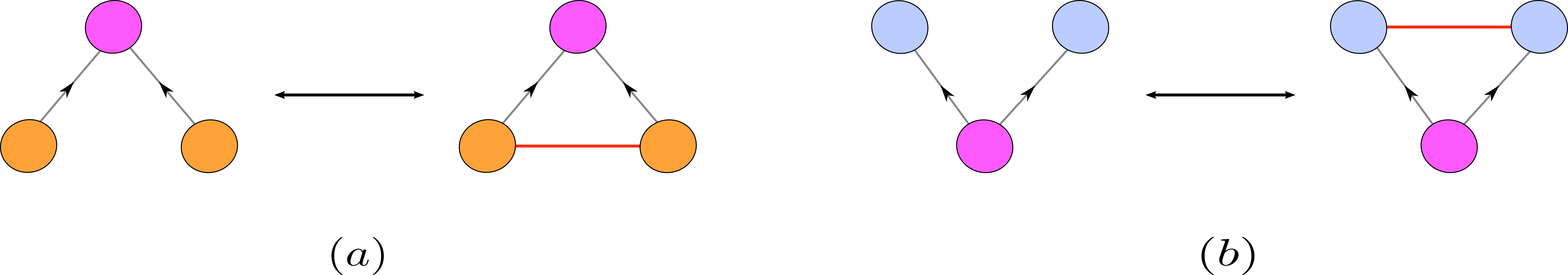
FIGURE 8.2: Relation between immediate incidence and (co)adjacency on the Hasse graph of a CC. (a): Two \((k-1)\) cells \(x^{k-1}\) and \(y^{k-1}\) (orange vertices) are 1-adjacent if and only if there exists a \(k\)-cell \(z^k\) (pink vertex) that is incident to \(x^{k-1}\) and \(y^{k-1}\). (b): Two \((k+1)\) cells \(x^{k+1}\) and \(y^{k+1}\) (blue vertices) are 1-coadjacent if and only if there exists a \(k\)-cell \(z^k\) (pink vertex) that is incident to \(x^{k+1}\) and \(y^{k+1}\).
8.1.2 Augmented Hasse graphs
The Hasse graph of a CC is useful because it shows that computations for a higher-order deep learning model can be reduced to computations for a graph-based model. Particularly, a \(k\)-cochain (signal) being processed on a CC \(\mathcal{X}\) can be thought as a signal on the corresponding vertices of the associated Hasse graph \(\mathcal{H}_{\mathcal{X}}\). The edges specified by the matrices \(B_{k,k+1}\) determine the message-passing structure of a given higher-order model defined on \(\mathcal{X}\). However, the message-passing structure determined via the matrices \(A_{r,k}\) is not directly supported on the corresponding edges of \(\mathcal{H}_{\mathcal{X}}\). Thus, it is sometimes desirable to augment the Hasse graph with additional edges other than the ones specified by the poset partial order relation of the CC. Along these lines, Definition 8.2 introduces the notion of augmented Hasse graph.
Definition 8.2 (Augmented Hasse graph) Let \(\mathcal{X}\) be a CC, and let \(\mathcal{H}_{\mathcal{X}}\) be its Hasse graph with vertex set \(V(\mathcal{H}_{\mathcal{X}})\) and edge set \(E(\mathcal{H}_{\mathcal{X}})\). Let \(\mathcal{N}=\{\mathcal{N}_1,\ldots,\mathcal{N}_n\}\) be a set of neighborhood functions defined on \(\mathcal{X}\). We say that \(\mathcal{H}_{\mathcal{X}}\) has an augmented edge \(e_{x,y}\) induced by \(\mathcal{N}\) if there exist \(\mathcal{N}_i \in \mathcal{N}\) such that \(x \in \mathcal{N}_i(y)\) or \(y \in \mathcal{N}_i(x)\). Denote by \(E_{\mathcal{N}}\) the set of all augmented edges induced by \(\mathcal{N}\). The augmented Hasse graph of \(\mathcal{X}\) induced by \(\mathcal{N}\) is defined to be the graph \(\mathcal{H}_{\mathcal{X}}(\mathcal{N})= (V(\mathcal{H}_{\mathcal{X}}), E(\mathcal{H}_{\mathcal{X}}) \cup E_{\mathcal{N}})\).
It is easier to think of the augmented Hasse graph in Definition 8.2 in terms of the matrices \(\mathbf{G}=\{G_1,\ldots,G_n\}\) associated with the neighborhood functions \(\mathcal{N}=\{\mathcal{N}_1,\ldots,\mathcal{N}_n\}\). Each augmented edge in \(\mathcal{H}_{\mathcal{X}}(\mathcal{N})\) corresponds to a non-zero entry in some \(G_i\in \mathbf{G}\). Since \(\mathcal{N}\) and \(\mathbf{G}\) store equivalent information, we use \(\mathcal{H}_{\mathcal{X}}(\mathbf{G})\) to denote the augmented Hasse graph induced by the edges determined by \(\mathbf{G}\). For instance, the graph given in Figure 8.1(c) is denoted by \(\mathcal{H}_{\mathcal{X}}( A_{0,1},coA_{2,1})\).
8.1.3 Reducibility of CCNNs to graph-based models
In this section, we show that any CCNN-based computational model can be realized as a message-passing scheme over a subgraph of the augmented Hasse graph of the underlying CC. Every CCNN is determined via a computational tensor diagram, which can be built using the elementary tensor operations, namely push-forward operations, merge nodes and split nodes. Thus, the reducibility of CCNN-based computations to message-passing schemes over graphs can be achieved by proving that these three tensor operations can be executed on an augmented Hasse graph. Proposition 8.2 states that push-forward operations are executable on augmented Hasse graphs.
Proposition 8.2 (Computation over augmented Hasse graph) Let \(\mathcal{X}\) be a CC and let \(\mathcal{F}_G \colon \mathcal{C}^i(\mathcal{X})\to \mathcal{C}^j(\mathcal{X})\) be a push-forward operator induced by a cochain map \(G\colon\mathcal{C}^i(\mathcal{X})\to \mathcal{C}^j(\mathcal{X})\). Any computation executed via \(\mathcal{F}_G\) can be reduced to a corresponding computation over the augmented Hassed graph \(\mathcal{H}_{\mathcal{X}}(G)\) of \(\mathcal{X}\).
Proof. Let \(\mathcal{X}\) be a CC. Let \(\mathcal{H}_{\mathcal{X}}(G)\) be the augmented Hasse graph of \(\mathcal{X}\) determined by \(G\). The definition of the augmented Hasse graph implies that there is a one-to-one correspondence between the vertices \(\mathcal{H}_{\mathcal{X}}(G)\) and the cells in \(\mathcal{X}\). Given a cell \(x\in \mathcal{X}\), let \(x^{\prime}\) be the corresponding vertex in \(\mathcal{H}_{\mathcal{X}}(G)\). Let \(y\) be a cell in \(\mathcal{X}\) with a feature vector \(\mathbf{h}_y\) computed via the push-forward operation specified by Equation (5.2). Recall that the vector \(\mathbf{h}_y\) is computed by aggregating all vectors \(\mathbf{h}_x\) attached to the neighbors \(x \in \mathcal{X}^i\) of \(y\) with respect to the neighborhood function \(\mathcal{N}_{G^T}\). Let \(m_{x,y}\) be a computation (message) that is executed between two cells \(x\) and \(y\) of \(\mathcal{X}\) as a part of the computation of push-forward \(\mathcal{F}_G\). It follows from the augmented Hasse graph definition that the cells \(x\) and \(y\) must have a corresponding non-zero entry in matrix \(G\). Moreover, this non-zero entry corresponds to an edge in \(\mathcal{H}_{\mathcal{X}}(G)\) between \(x^{\prime}\) and \(y^{\prime}\). Thus, the computation \(m_{x,y}\) between the cells \(x\) and \(y\) of \(\mathcal{X}\) can be carried out as the computation (message) \(m_{x^{\prime},y^{\prime}}\) between the corresponding vertices \(x^{\prime}\) and \(y^{\prime}\) of \(\mathcal{H}_{\mathcal{X}}(G)\).
Similarly, computations on an arbitrary merge node can be characterized in terms of computations on a subgraph of the augmented Hasse graph of the underlying CC. Proposition 8.3 formalizes this statement.
Proposition 8.3 (Reduction of merge node to augmented Hasse graph) Any computation executed via a merge node \(\mathcal{M}_{\mathbf{G},\mathbf{W}}\) as given in Equation (5.1) can be reduced to a corresponding computation over the augmented Hasse graph \(\mathcal{H}_{\mathcal{X}}(\mathbf{G})\) of the underlying CC.
Proof. Let \(\mathcal{X}\) be a CC. Let \(\mathbf{G}=\{ G_1,\ldots,G_n\}\) be a sequence of cochain operators defined on \(\mathcal{X}\). Let \(\mathcal{H}_{\mathcal{X}}(\mathbf{G})\) be the augmented Hasse graph determined by \(\mathbf{G}\). By the augmented Hasse graph definition, there is a one-to-one correspondence between the vertices of \(\mathcal{H}_{\mathcal{X}}(\mathbf{G})\) and the cells of \(\mathcal{X}\). For each cell \(x\in \mathcal{X}\), let \(x^{\prime}\) be the corresponding vertex in \(\mathcal{H}_{\mathcal{X}}(\mathbf{G})\). Let \(m_{x,y}\) be a computation (message) that is executed between two cells \(x\) and \(y\) of \(\mathcal{X}\) as part of the evaluation of function \(\mathcal{M}_{\mathbf{G},W}\). Hence, the two cells \(x\) and \(y\) must have a corresponding non-zero entry in a matrix \(G_i\in\mathbf{G}\). By the augmented Hasse graph definition, this non-zero entry corresponds to an edge in \(\mathcal{H}_{\mathcal{X}}(\mathbf{G})\) between \(x^{\prime}\) and \(y^{\prime}\). Thus, the computation \(m_{x,y}\) between the cells \(x\) and \(y\) of \(\mathcal{X}\) can be carried out as the computation (message) \(m_{x^{\prime},y^{\prime}}\) between the corresponding vertices \(x^{\prime}\) and \(y^{\prime}\) of \(\mathcal{H}_{\mathcal{X}}(\mathbf{G})\).
Propositions 8.2 and 8.3 ensure that push-forward and merge node computations can be realized on augmented Hasse graphs. Theorem 8.1 generalizes Propositions 8.2 and 8.3, stating that any computation on tensor diagrams is realizable on augmented Hasse graphs.
Theorem 8.1 (Reduction of tensor diagram to augmented Hasse graph) Any computation executed via a tensor diagram \(\mbox{CCNN}_{\mathbf{G};\mathbf{W}}\) can be reduced to a corresponding computation on the augmented Hasse graph \(\mathcal{H}_{\mathcal{X}}(\mathbf{G})\).
Proof. The conclusion follows directly from Propositions 8.3 and 8.2, along with the fact that any tensor diagram can be realized in terms of the three elementary tensor operations.
According to Theorem 8.1, a tensor diagram and its corresponding augmented Hasse graph encode the same computations in alternative forms. Figure 8.3 illustrates that the augmented Hasse graph provides a computational summary of the associated tensor diagram representation of a CCNN.
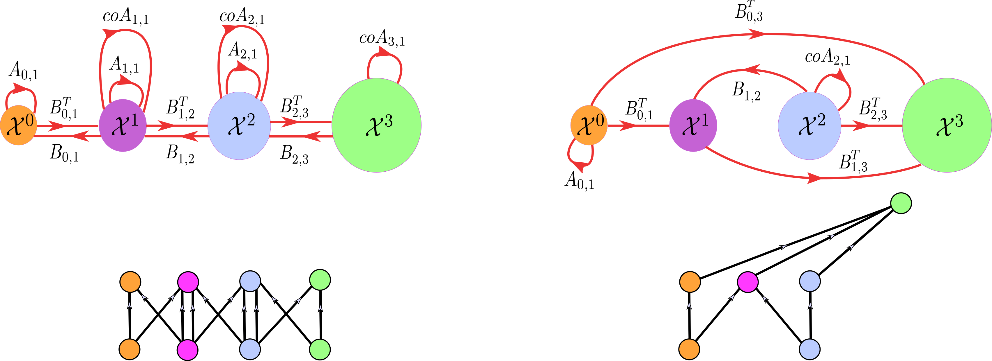
FIGURE 8.3: Tensor diagrams of two CCNNs and their corresponding augmented Hasse graphs. Edge labels are dropped from the tensor diagrams to avoid clutter, as they can be inferred from the corresponding augmented Hasse graphs. (a): A tensor diagram obtained from a higher-order message-passing scheme. (b): A tensor diagram obtained by using the three elementary tensor operations.
8.1.4 Augmented Hasse graphs and CC-pooling
The Hasse graph and its augmented version are graph representations of the poset structure of the underlying CC. It is instructive to interpret the (un)pooling operations (Definitions 7.1 and 7.2) with respect to these graphs. The CC-pooling operation of Definition 7.1 maps a signal in the poset structure from lower-rank cells to higher-rank ones. On the other hand, the CC-unpooling operation of Definition 7.2 maps a signal in the opposite direction. Figure 8.4 presents an example of CC (un)-pooling operations visualized over the augmented Hasse graph of the underlying CC.
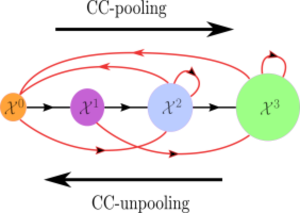
FIGURE 8.4: CC (un)-pooling operations viewed on the augmented Hasse graph of a CC. The vertices in the figure represent skeletons in the underlying CC. Black edges represent edges in the Hasse graph between these vertices, whereas red edges represent edges obtained from the augmented Hasse graph structure. CC-pooling corresponds to pushing a signal in the poset structure from lower-rank to higher-rank vertices, whereas CC-unpooling corresponds to pushing a signal in the poset structure from higher-rank to lower-rank vertices.
8.1.5 Augmented Hasse diagrams, message passing and merge nodes
The difference between constructing a CCNN using the higher-order message passing paradigm given in Section 6.1 versus using the three elementary tensor operations given in Section 5.3 has been demonstrated in Section 6.3. In particular, Section 6.3 mentions that merge nodes naturally allow for a more flexible computational framework in comparison to the higher-order message-passing paradigm. This flexibility manifests in terms of the underlying tensor diagram as well as the input for the network under consideration. The difference between tensor operations and higher-order message passing can also be highlighted with augmented Hasse graphs, as demonstrated in Figure 8.3. Figure 8.3(a) shows a tensor diagram obtained from a higher-order message-passing scheme on a CCNN. We observe two key properties of this CCNN: the initial input cochains are supported on all cells of all dimensions of the domain, and the CCNN updates all cochains supported on all cells of all dimensions of the domain at every iteration given a predetermined set of neighborhood functions. As a consequence, the corresponding augmented Hasse graph exhibits a uniform topological structure. In contrast, Figure 8.3(b) shows a tensor diagram constructed using the three elementary tensor operations. As the higher-order message-passing rules do not impose constraints, the resulting augmented Hasse graph exhibits a more flexible structure.
8.1.6 Higher-order representation learning
The relation between augmented Hasse graphs and CCs given by Theorem 8.1 suggests that many graph-based deep learning constructions have analogous constructions for CCs. In this section, we demonstrate how higher-order representation learning can be reduced to graph representation learning (Hamilton, Ying, and Leskovec 2017), as an application of certain CC computations as augmented Hasse graph computations.
The goal of graph representation is to learn a mapping that embeds the vertices, edges or subgraphs of a graph into a Euclidean space, so that the resulting embedding captures useful information about the graph. Similarly, higher-order representation learning (Hajij, Istvan, and Zamzmi 2020) involves learning an embedding of various cells in a given topological domain into a Euclidean space, preserving the main structural properties of the topological domain. More precisely, given a complex \(\mathcal{X}\), higher-order representation learning refers to learning a pair \((enc, dec)\) of functions, consisting of the encoder map \(enc \colon \mathcal{X}^k \to \mathbb{R}^d\) and the decoder map \(dec \colon \mathbb{R}^d \times \mathbb{R}^d \to \mathbb{R}\). The encoder function associates to every \(k\)-cell \(x^k\) in \(\mathcal{X}\) a feature vector \(enc(x^k)\), which encodes the structure of \(x^k\) with respect to the structures of other cells in \(\mathcal{X}\). On the other hand, the decoder function associates to every pair of cell embeddings a measure of similarity, which quantifies some notion of relation between the corresponding cells. We optimize the trainable functions \((enc, dec)\) using a context-specific similarity measure \(sim \colon \mathcal{X}^k \times \mathcal{X}^k \to \mathbb{R}\) and an objective function \[\begin{equation} \mathcal{L}_k=\sum_{ x^k \in \mathcal{X}^k } l( dec( enc(x^{k}), enc(y^{k})),sim(x^{k},y^k)), \tag{8.1} \end{equation}\] where \(l \colon \mathbb{R} \times \mathbb{R} \to \mathbb{R}\) is a loss function. The precise relation between higher-order and graph representation learning is given by Proposition 8.4.
Proposition 8.4 (Higher-order representation learning as graph representation learning) Higher-order representation learning can be reduced to graph representation learning.
Proof. Let \(sim\colon \mathcal{X}^k \times \mathcal{X}^k \to \mathbb{R}\) be a similarity measure. The graph \(\mathcal{G}_{\mathcal{X}^k}\) is defined as the graph whose vertex set corresponds to cells in \(\mathcal{X}^k\) and whose edges correspond to cell pairs in \(\mathcal{X}^k \times \mathcal{X}^k\) mapped to non-zero values by the function \(sim\). Thus, the pair \((enc, dec)\) corresponds to a pair \((enc_{\mathcal{G}}, dec_{\mathcal{G}})\) of the form \(enc_{\mathcal{G}}\colon \mathcal{G}_{\mathcal{X}^k} \to \mathbb{R}\) and \(dec_{\mathcal{G}}\colon \mathbb{R}^d \times \mathbb{R}^d \to \mathbb{R}\). Thereby, learning the pair \((enc, dec)\) is reduced to learning the pair \((enc_{\mathcal{G}}, dec_{\mathcal{G}})\).
TopoEmbedX, one of our three contributed software packages, supports higher-order representation learning on cell complexes, simplicial complexes, and CCs. The main computational principle underlying TopoEmbedX is Proposition 8.4. Specifically, TopoEmbedX converts a given higher-order domain into a subgraph of the corresponding augmented Hasse graph, and then utilizes existing graph representation learning algorithms to compute the embedding of elements of this subgraph. Given the correspondence between the elements of the augmented Hasse graph and the original higher-order domain, this results in obtaining embeddings for the higher-order domain.
Remark. Following our discussion on Hasse graphs, and particularly the ability to transform computations on a CCNN to computations on a (Hasse) graph, one may argue that GNNs are sufficient and that there is no need for CCNNs. However, this is a misleading clue, in the sense that any computation can be represented by a computational graph. Applying a standard GNN over the augmented Hasse graph of a CC is not equivalent to applying a CCNN. This point will become clearer in Section 8.2, where we introduce CCNN equivariances.
8.2 On the equivariance of CCNNs
Analogous to their graph counterparts, higher-order deep learning models, and CCNNs in particular, should always be considered in conjunction with their underlying equivariance (Bronstein et al. 2021). We now provide novel definitions for permutation and orientation equivariance for CCNNs and draw attention to their relations with conventional notions of equivariance defined for GNNs.
8.2.1 Permutation equivariance of CCNNs
Motivated by Proposition 8.1, which characterizes the structure of a CC, this section introduces permutation-equivariant CCNNs. We first define the action of the permutation group on the space of cochain maps.
Definition 8.3 (Permutation action on space of cochain maps) Let \(\mathcal{X}\) be a CC. Define \(\mbox{Sym}(\mathcal{X}) = \prod_{i=0}^{\dim(\mathcal{X})} \mbox{Sym}(\mathcal{X}^k)\) the group of rank-preserving permutations of the cells of \(\mathcal{X}\). Let \(\mathbf{G}=\{G_k\}\) be a sequence of cochain maps defined on \(\mathcal{X}\) with \(G_k \colon \mathcal{C}^{i_k}\to \mathcal{C}^{j_k}\), \(0\leq i_k,j_k\leq \dim(\mathcal{X})\). Let \(\mathcal{P}=(\mathbf{P}_i)_{i=0}^{\dim(\mathcal{X})} \in \mbox{Sym}(\mathcal{X})\). Define the permutation (group) action of \(\mathcal{P}\) on \(\mathbf{G}\) by \(\mathcal{P}(\mathbf{G}) = (\mathbf{P}_{j_k} G_{k} \mathbf{P}_{i_k}^T )_{i=0}^{\dim(\mathcal{X})}\).
We introduce permutation-equivariant CCNNs in Definition 8.4, using the group action given in Definition 8.3. Definition 8.4 generalizes the relevant definitions in (T. Mitchell Roddenberry, Glaze, and Segarra 2021; Schaub et al. 2021). We refer the reader to (Jogl 2022; Veličković 2022) for a related discussion. Hereafter, we use \(\mbox{Proj}_k \colon \mathcal{C}^1\times \cdots \times \mathcal{C}^m \to \mathcal{C}^k\) to denote the standard \(k\)-th projection for \(1\leq k \leq m\), defined via \(\mbox{Proj}_k ( \mathbf{H}_{1},\ldots, \mathbf{H}_{k},\ldots,\mathbf{H}_{m})= \mathbf{H}_{k}\).
Definition 8.4 (Permutation-equivariant CCNN) Let \(\mathcal{X}\) be a CC and let \(\mathbf{G}= \{G_k\}\) be a finite sequence of cochain maps defined on \(\mathcal{X}\). Let \(\mathcal{P}=(\mathbf{P}_i)_{i=0}^{\dim(\mathcal{X})} \in \mbox{Sym}(\mathcal{X})\). A CCNN of the form \[\begin{equation*} \mbox{CCNN}_{\mathbf{G};\mathbf{W}}\colon \mathcal{C}^{i_1}\times\mathcal{C}^{i_2}\times \cdots \times \mathcal{C}^{i_m} \to \mathcal{C}^{j_1}\times\mathcal{C}^{j_2}\times \cdots \times \mathcal{C}^{j_n} \end{equation*}\] is called a permutation-equivariant CCNN if \[\begin{equation} \mbox{Proj}_k \circ \mbox{CCNN}_{\mathbf{G};\mathbf{W}}(\mathbf{H}_{i_1},\ldots ,\mathbf{H}_{i_m})= \mathbf{P}_{k} \mbox{Proj}_k \circ \mbox{CCNN}_{\mathcal{P}(\mathbf{G});\mathbf{W}}(\mathbf{P}_{i_1} \mathbf{H}_{i_1}, \ldots ,\mathbf{P}_{i_m} \mathbf{H}_{i_m}) \end{equation}\] for all \(1 \leq k\leq m\) and for any \((\mathbf{H}_{i_1},\ldots ,\mathbf{H}_{i_m}) \in\mathcal{C}^{i_1}\times\mathcal{C}^{i_2}\times \cdots \times \mathcal{C}^{i_m}\).
Definition 8.4 generalizes the corresponding notion of permutation equivariance of GNNs. Consider a graph with \(n\) vertices and adjacency matrix \(A\). Denote a GNN on this graph by \(\mathrm{GNN}_{A;W}\). Let \(H \in \mathbb{R}^{n \times k}\) be vertex features. Then \(\mathrm{GNN}_{A;W}\) is permutation equivariant in the sense that for \(P \in \mbox{Sym}(n)\) we have \(P \,\mathrm{GNN}_{A;W}(H) = \mathrm{GNN}_{PAP^{T};W}(PH)\).
In general, working with Definition 8.4 may be cumbersome. It is easier to characterize the equivariance in terms of merge nodes. To this end, recall that the height of a tensor diagram is the longest path from any source node to any target node. Proposition 8.5 allows us to express tensor diagrams of height one in terms of merge nodes.
Proposition 8.5 (Tensor diagrams of height one as merge nodes) Let \(\mbox{CCNN}_{\mathbf{G};\mathbf{W}}\colon \mathcal{C}^{i_1}\times\mathcal{C}^{i_2}\times \cdots \times \mathcal{C}^{i_m} \to \mathcal{C}^{j_1}\times\mathcal{C}^{j_2}\times \cdots \times \mathcal{C}^{j_n}\) be a CCNN with a tensor diagram of height one. Then \[\begin{equation} \label{merge_lemma} \mbox{CCNN}_{\mathbf{G};\mathbf{W}}=( \mathcal{M}_{\mathbf{G}_{j_1};\mathbf{W}_1},\ldots, \mathcal{M}_{\mathbf{G}_{j_n};\mathbf{W}_n}), \tag{8.2} \end{equation}\] where \(\mathbf{G}_k \subseteq \mathbf{G}\).
Proof. Let \(\mbox{CCNN}_{\mathbf{G};\mathbf{W}}\colon \mathcal{C}^{i_1}\times\mathcal{C}^{i_2}\times \cdots \times \mathcal{C}^{i_m} \to \mathcal{C}^{j_1}\times\mathcal{C}^{j_2}\times \cdots \times \mathcal{C}^{j_n}\) be a CCNN with a tensor diagram of height one. Since the codomain of the function \(\mbox{CCNN}_{\mathbf{G};\mathbf{W}}\) is \(\mathcal{C}^{j_1}\times\mathcal{C}^{j_2}\times \ldots \times \mathcal{C}^{j_n}\), then \(\mbox{CCNN}_{\mathbf{G};\mathbf{W}}\) is determined by \(n\) functions \(F_k\colon \mathcal{C}^{i_1}\times\mathcal{C}^{i_2}\times \cdots \times \mathcal{C}^{i_m} \to \mathcal{C}^{j_k}\) for \(1 \leq k \leq n\). Since the height of the tensor diagram of \(\mbox{CCNN}_{\mathbf{G};\mathbf{W}}\) is one, then each function \(F_k\) is also of height one and it is thus a merge node by definition. The result follows.
Proposition 8.5 states that every target node \(j_k\) in a tensor diagram of height one is a merge node specified by the operators \(\mathbf{G}_{j_k}\) formed by the labels of the edges with target \(j_k\). Definition 8.4 introduces the general notion of permutation equivariance of CCNNs. Definition 8.5 introduces the notion of permutation-equivariant merge node. Since a merge node is a CCNN, Definition 8.5 is a special case of Definition 8.4.
Definition 8.5 (Permutation-equivariant merge node) Let \(\mathcal{X}\) be a CC and let \(\mathbf{G}= \{G_k\}\) be a finite sequence of cochain operators defined on \(\mathcal{X}\) with \(G_k\colon C^{i_k}(\mathcal{X})\to C^{j}(\mathcal{X})\). Let \(\mathcal{P}=(\mathbf{P}_i)_{i=0}^{\dim(\mathcal{X})} \in \mbox{Sym}(\mathcal{X})\). We say that the merge node given in Equation (5.1) is a permutation-equivariant merge node if \[\begin{equation} \mathcal{M}_{\mathbf{G};\mathbf{W}}(\mathbf{H}_{i_1},\ldots ,\mathbf{H}_{i_m})= \mathbf{P}_{j} \mathcal{M}_{\mathcal{P}(\mathbf{G});\mathbf{W}}(\mathbf{P}_{i_1} \mathbf{H}_{i_1}, \ldots ,\mathbf{P}_{i_1} \mathbf{H}_{i_m}) \end{equation}\] for any \((\mathbf{H}_{i_1},\ldots ,\mathbf{H}_{i_m}) \in \mathcal{C}^{i_1}\times\mathcal{C}^{i_2}\times \cdots \times \mathcal{C}^{i_m}\).
Proposition 8.6 (Permutation-equivariant CCNN of height one and merge nodes) Let \(\mbox{CCNN}_{\mathbf{G};\mathbf{W}}\colon \mathcal{C}^{i_1}\times\mathcal{C}^{i_2}\times \cdots \times \mathcal{C}^{i_m} \to \mathcal{C}^{j_1}\times\mathcal{C}^{j_2}\times \cdots \times \mathcal{C}^{j_n}\) be a CCNN with a tensor diagram of height one. Then \(\mbox{CCNN}_{\mathbf{G};\mathbf{W}}\) is permutation equivariant if and only the merge nodes \(\mathcal{M}_{\mathbf{G}_{j_k};\mathbf{W}_k}\) given in Equation (8.2) are permutation equivariant for \(1 \leq k \leq n\).
Proof. If a CCNN is of height one, then by Proposition 8.5, \(\mbox{Proj}_k \circ \mbox{CCNN}_{\mathbf{G};\mathbf{W}}(\mathbf{H}_{i_1},\ldots ,\mathbf{H}_{i_m})= \mathcal{M}_{\mathbf{G}_{j_k};\mathbf{W}_k}\). Hence, the result follows from the definition of merge node permutation equivariance (Definition 8.5) and the definition of CCNN permutation equivariance (Definition 8.4).
Finally, Theorem 8.2 characterizes the permutation equivariance of CCNNs in terms of merge nodes. From this point of view, Theorem 8.2 provides a practical version of permutation equivariance for CCNNs.
Theorem 8.2 (Permutation-equivariant CCNN and merge nodes) A \(\mbox{CCNN}_{\mathbf{G};\mathbf{W}}\) is permutation equivariant if and only if every merge node in \(\mbox{CCNN}_{\mathbf{G};\mathbf{W}}\) is permutation equivariant.
Proof. Proposition 8.6 proves this fact for CCNNs of height one. For CCNNs of height \(n\), it is enough to observe that a CCNN of height \(n\) is a composition of \(n\) CCNNs of height one and that the composition of two permutation-equivariant networks is a permutation-equivariant network.
Remark. Our permutation equivariance assumes that all cells in each dimension are independently labeled with indices. However, if we label the cells in a CC with subsets of the powerset \(\mathcal{P}(S)\) rather than with indices, then we only need to consider permutations of the powerset that are induced by permutations of the 0-cells in order to ensure permutation equivariance.
Remark. A GNN is equivariant in that a permutation of the vertex set of the graph and the input signal over the vertex set yields the same permutation of the GNN output. Applying a standard GNN over the augmented Hasse graph of the underlying CC is thus not equivalent to applying a CCNN. Although the message-passing structures are the same, the weight-sharing and permutation equivariance of the standard GNN and CCNN are different. In particular, Definition 4.2 gives additional structure, which is not preserved by an arbitrary permutation of the vertices in the augmented Hasse graph. Thus, care is required in order to reduce message passing over a CCNN to message passing over the associated augmented Hasse graph. Specifically, one need only consider the subgroup of permutations of vertex labels in the augmented Hasse graph which are induced by permutations of 0-cells in the corresponding CC. Thus, there is merit in adopting the rich notions of topology to think about distributed, structured learning architectures, as topological constructions facilitate reasoning about computation in ways that are not within the scope of graph-based approaches.
Remark. Note that Proposition 8.4 does not contradict the previous remark. In fact, the computations described in Proposition 8.4 are conducted on a particular subgraph of the Hasse graph whose vertices are the \(k\)-cells of the underlying complex. Differences between graph-based networks and TDL networks start to emerge particularly once different dimensions are considered simultaneously during computations.
8.2.2 Orientation equivariance of CCNNs
When CC are reduced to regular cell complexes, then orientation equivariance can also be introduced to CCNNs. Analogous to Definition 8.3, we introduce the following definition of orientation actions on CCs.
Definition 8.6 (Orientation action on space of diagonal-cochain maps) Let \(\mathcal{X}\) be a CC. Let \(\mathbf{G}=\{G_k\}\) be a sequence of cochain operators defined on \(\mathcal{X}\) with \(G_k \colon \mathcal{C}^{i_k}\to \mathcal{C}^{j_k}\), \(0\leq i_k,j_k\leq \dim(\mathcal{X})\). Let \(O(\mathcal{X})\) be the group of tuples \(\mathcal{D}=(\mathbf{D}_i)_{i=0}^{\dim(\mathcal{X})}\) of diagonal matrices with diagonals \(\pm 1\) of size \(|\mathcal{X}^k| \times |\mathcal{X}^k|\) such that \(\mathbf{D}_0=I\). Define the orientation (group) action of \(\mathcal{D}\) on \(\mathbf{G}\) by \(\mathcal{D}(\mathbf{G}) = (\mathbf{D}_{j_k} G_{k} \mathbf{D}_{i_k})_{i=0}^{\dim(\mathcal{X})}\).
We introduce orientation-equivariant CCNNs in Definition 8.7, using the group action given in Definition 8.6. Orientation equivariance for CCNNs (Definition 8.7) is put forward in analogous way to permutation equivariance for CCNNs (Definition 8.4).
Definition 8.7 (Orientation-equivariant CCNN) Let \(\mathcal{X}\) be a CC and let \(\mathbf{G}= \{G_k\}\) be a finite sequence of cochain operators defined on \(\mathcal{X}\). Let \(\mathcal{D} \in O(\mathcal{X})\). A CCNN of the form \[\begin{equation*} \mbox{CCNN}_{\mathbf{G};\mathbf{W}}\colon \mathcal{C}^{i_1}\times\mathcal{C}^{i_2}\times \cdots \times \mathcal{C}^{i_m} \to \mathcal{C}^{j_1}\times\mathcal{C}^{j_2}\times \cdots \times \mathcal{C}^{j_n} \end{equation*}\] is called an orientation-equivariant CCNN if \[\begin{equation} \mbox{Proj}_k \circ \mbox{CCNN}_{\mathbf{G};\mathbf{W}}(\mathbf{H}_{i_1},\ldots ,\mathbf{H}_{i_m})=\mathbf{D}_{k} \mbox{Proj}_k \circ \mbox{CCNN}_{\mathcal{D}(\mathbf{G});\mathbf{W}}((\mathbf{D}_{i_1} \mathbf{H}_{i_1}, \ldots ,\mathbf{D}_{i_1} \mathbf{H}_{i_m})) \end{equation}\] for all \(1 \leq k\leq m\) and for any \((\mathbf{H}_{i_1},\ldots ,\mathbf{H}_{i_m}) \in \mathcal{C}^{i_1}\times\mathcal{C}^{i_2}\times \cdots \times \mathcal{C}^{i_m}\).
Propositions 8.5 and 8.6 can be stated analogously for the orientation equivariance case. We skip stating these facts here, and only state the main theorem that characterizes the orientation equivariance of CCNNs in terms of merge nodes.
Theorem 8.3 (Orientation-equivariant CCNN and merge nodes) A \(\mbox{CCNN}_{\mathbf{G};\mathbf{W}}\) is orientation equivariant if and only if every merge node in \(\mbox{CCNN}_{\mathbf{G};\mathbf{W}}\) is orientation equivariant.
References
For related structures (e.g., simplicial/cell complexes), this poset is typically called the face poset (Wachs 2006).↩︎