Chapter 4 Combinatorial complexes
This section introduces combinatorial complexes (CCs), a novel class of higher-order domains that generalizes graphs, simplicial complexes, cell complexes, and hypergraphs. Figure 4.1 shows a first illustration of the generalization that CCs provide over such domains. Moreover, Table 4.1 enlists the relation-related features of higher-order domains and graphs, thus summarizing the relation-related generalization attained by CCs.
FIGURE 4.1: Illustration of how CCs generalize various domains. (a): A set \(S\) consists of abstract entities (vertices) with no relations. (b): A graph models binary relations between its vertices (i.e., elements of \(S\)). (c): A simplicial complex models a hierarchy of higher-order relations (i.e., relations between the relations) but with rigid constraints on the ‘shape’ of its relations. (d): Similar to simplicial complexes, a cell complex models a hierarchy of higher-order relations, but with more flexibility in the shape of the relations (i.e., ‘cells’). (f): A hypergraph models arbitrary set-type relations between elements of \(S\), but these relations do not have a hierarchy among them. (e): A CC combines features of cell complexes (hierarchy among its relations) and of hypergraphs (arbitrary set-type relations), generalizing both domains.
| Relation-related features | CC | Hypergraph | Cell complex | Simplicial complex |
|---|---|---|---|---|
| Hierarcy of relations | √ | √ | √ | |
| Set-type relations | √ | √ | ||
| Multi-relation coupling | √ | √ | √ | |
| Rank not cardinality | √ | √ | √ |
In Section 4.1, we introduce the definition of CC and provide examples of CCs. In Section 4.2, we define the notion of CC-homomorphism and present relevant examples. In Section 4.3, we present the motivation behind the CC structure from a practical point of view. In Section 4.4, we demonstrate the computational version of neighborhood functions on neighborhood matrices. Finally, in Section 4.5, we introduce the notion of CC-cochain.
4.1 CC definition
We seek to define a structure that bridges the gap between simplicial/cell complexes and hypergraphs, as discussed in Section 3.3. To this end, we introduce the combinatorial complex (CC), a higher-order domain that can be viewed from three perspectives: as a simplicial complex whose cells and simplices are allowed to be missing; as a generalized cell complex with relaxed structure; or as a hypergraph enriched through the inclusion of a rank function.
Definition 4.1 (Combinatorial complex) A combinatorial complex (CC) is a triple \((S, \mathcal{X}, \mbox{rk})\) consisting of a set \(S\), a subset \(\mathcal{X}\) of \(\mathcal{P}(S)\setminus\{\emptyset\}\), and a function \(\mbox{rk} \colon \mathcal{X}\to \mathbb{Z}_{\ge 0}\) with the following properties:
- for all \(s\in S\), \(\{s\}\in\mathcal{X}\), and
- the function \(\mbox{rk}\) is order-preserving, which means that if \(x,y\in \mathcal{X}\) satisfy \(x\subseteq y\), then \(\mbox{rk}(x) \leq \mbox{rk}(y)\).
Elements of \(S\) are called entities or vertices, elements of \(\mathcal{X}\) are called relations or cells, and \(\mbox{rk}\) is called the rank function of the CC.
For brevity, \(\mathcal{X}\) is used as shorthand notation for a CC \((S,\mathcal{X},\mbox{rk})\). Definition 4.1 sets up a framework to construct higher-order networks upon which we can define general purpose higher-order deep learning architectures. Observe that CCs exhibit both hierarchical and set-type relations. Particularly, the rank function \(\mbox{rk}\) of a CC induces a hierarchy of relations in the CC. Further, CCs encompass set-type relations as there are no relation constraints in Definition 4.1. Thus, CCs subsume cell complexes and hypergraphs in the sense that they combine the relation-related features of both. Table 4.1 provides a comparative summary of relation-related features among CCs and common higher-order networks and graphs.
Remark. We typically require that \(\mbox{rk}(\{s\})=0\) for each singleton cell \(\{s\}\) in a CC. Such a convention aligns CCs naturally with simplicial and cellular complexes.
The rank of a cell \(x\in\mathcal{X}\) is the value \(\mbox{rk}(x)\) of the rank function \(\mbox{rk}\) at \(x\). The dimension \(\mbox{dim}(\mathcal{X})\) of a CC \(\mathcal{X}\) is the maximal rank among its cells. A cell of rank \(k\) is called a \(k\)-cell and is denoted by \(x^k\). The \(k\)-skeleton of a CC \(\mathcal{X}\), denoted \(\mathcal{X}^{(k)}\), is the set of cells of rank at most \(k\) in \(\mathcal{X}\). The set of cells of rank exactly \(k\) is denoted by \(\mathcal{X}^k\). Note that this set corresponds to \(\mathcal{X}^k=\mbox{rk}^{-1}(\{k\})\). The \(1\)-cells are called the edges of \(\mathcal{X}\). In general, an edge of a CC may contain more than two nodes. CCs whose edges have exactly two nodes are called graph-based CCs. In this paper, we primarily work with graph-based CCs.
Example 4.1 (CCs of dimension two and three) Figure 4.2 shows four examples of CCs. For instance, Figure 4.2(a) shows a 2-dimensional CC on a vertex set \(S=\{s_0,s_1,s_2\}\), consisting of \(0\)-cells \(\{s_0\}\), \(\{s_1\}\), and \(\{s_2\}\) (shown in orange), \(1\)-cell \(\{s_0, s_1\}\) (purple), and \(2\)-cell \(\{s_0, s_1, s_2\} = S\) (blue).
FIGURE 4.2: Examples of CCs. Orange circles represent vertices. Pink, blue, and green colors represent cells of rank one, two, and three, respectively. Each of the CCs in (a), (b), and (d) has dimension equal to two, whereas the CC in (c) has dimension equal to three.
4.2 CC-homomorphisms and sub-CCs
CC-homomorphisms are maps relating CCs to one another. CC-homomorphisms play an important role in delineating the process of lifting graphs or other higher-order domains to CCs. Intuitively, a lifting map is a well-defined procedure that converts a domain of certain type, such as a graph, to a domain of another type, such as a CC. The usefulness of lifting maps lie in their ability to enable the application of deep learning models defined on CCs to more common domains, such as graphs, cell complexes or simplicial complexes. We study lifting maps in detail and provide examples of them in Appendix B. Definition 4.2 formalizes the notion of CC-homomorphism.
Definition 4.2 (CC-homomorphism) A homomorphism from a CC \((S_1, \mathcal{X}_1, \mbox{rk}_1)\) to a CC \((S_2, \mathcal{X}_2, \mbox{rk}_2)\), also called a CC-homomorphism, is a function \(f \colon \mathcal{X}_1 \to \mathcal{X}_2\) that satisfies the following conditions:
- If \(x,y\in\mathcal{X}_1\) satisfy \(x\subseteq y\), then \(f(x) \subseteq f(y)\).
- If \(x\in\mathcal{X}_1\), then \(\mbox{rk}_1(x)\geq \mbox{rk}_2(f(x))\).
The second condition in Definition 4.2 assures that a CC-homomorphism may only map a \(k\)-cell in \(\mathcal{X}_1\) to a cell in \(\mathcal{X}_2\) with rank no greater than \(k\). When \(\mbox{rk}_1(x) = \mbox{rk}_2(f(x))\) for all \(x \in \mathcal{X}_1\) and \(f\) is injective, then we call the homomorphism \(f\) a CC-embedding. CC-embeddings are useful in practice as they can be used to ‘lift’ a domain, such as a graph, to a CC by augmenting that domain with higher-order cells. Example 4.2 displays three CC-embeddings, while Example 4.3 presents a CC-homomorphism that is not a CC-embedding.
Example 4.2 (CC-embeddings) Figures 4.3(a) and (b) show two CC-embeddings. In Figure 4.3(a), each cell in the graph on the left-hand side is sent to its corresponding cell in the CC on the right-hand side. Similarly, in Figure 4.3(b), each cell in the cell complex on the left is sent to its corresponding cell in the CC on the right. It is easy to verify that each of these two maps is a CC-embedding.
FIGURE 4.3: Examples of CC-homomorphisms. Pink, blue, and green colors represent cells of rank one, two, and three, respectively. (a): An embedding of a \(1\)-dimensional CC into a \(2\)-dimensional CC. (b): An embedding of a \(2\)-dimensional CC into a \(3\)-dimensional CC. (c) An example of a CC-homomorphism. The CC \(\mathcal{X}_1\) is on the left, \(\mathcal{X}_2\) is on the right, and the homomorphism \(f\) is represented by the black arrow. Intuitively, the CC-homomorphism \(f\) can be viewed as a combinatorial analogue to a continuous function between \(S_1 = \{1, 2, 3,4\}\) and \(S_2 = \{a, b, c\}\) that ‘collapses’ the cell \(\{1,2,3\}\) to the cell \(\{a,b\}\), and the cell \(\{1,2,3,4\}\) to the cell \(\{a,b,c\}\). Observe that CC-homomorphisms generalize simplicial maps [Munkres (2018)} from this perspective.
Example 4.3 (A CC-homomorphism) We present an example of a CC-homomorphism that is not a CC-embedding. Consider the sets \(S_1 = \{1, 2, 3,4\}\) and \(S_2 = \{a, b, c\}\). Let \(\mathcal{X}_1\) denote the CC on \(S_1\) consisting of one 3-cell \(\{1,2,3,4\}\), one 2-cell \(\{1,2,3\}\), and four 0-cells corresponding to the elements of \(S_1\). Likewise, let \(\mathcal{X}_2\) denote the CC on \(S_2\) consisting of one 3-cell \(\{a,b,c\}\), one 2-cell \(\{a,b\}\), and three 0-cells corresponding to the elements of \(S_2\). CCs \(\mathcal{X}_1\) and \(\mathcal{X}_2\) are visualized in Figure 4.3(c). Consider the function \(f \colon S_1 \to S_2\) defined as \(f(1) = f(2) = a,~f(3) = b\) and \(f(4) = c\). It is easy to verify that \(f\) induces a CC-homomorphism from \(\mathcal{X}_1\) to \(\mathcal{X}_2\).
Definition 4.3 (Sub-CC) Let \((S,\mathcal{X}, \mbox{rk})\) be a CC. A sub-combinatorial complex (sub-CC) of a CC \((S,\mathcal{X}, \mbox{rk})\) is a CC \((A,\mathcal{Y},\mbox{rk}^{\prime})\) such that \(A\subseteq S\), \(\mathcal{Y}\subseteq\mathcal{X}\) and \(\mbox{rk}^{\prime} = \mbox{rk}|_{\mathcal{Y}}\) is the restriction of \(\mbox{rk}\) on \(\mathcal{Y}\).
For brevity, we refer to the sub-CC \((A,\mathcal{Y},\mbox{rk}^{\prime})\) as \(\mathcal{Y}\). Any subset of \(A \subseteq S\) can be used to induce a sub-CC as follows. Consider the set \(\mathcal{X}_A = \{x \in \mathcal{X} \mid x \subseteq A\}\) together with the restriction \(\mbox{rk}|_{\mathcal{X}_A}\). It is easy to see that the triple \((A,\mathcal{X}_A,\mbox{rk}|_{\mathcal{X}_A})\) constitutes a CC, which we call the sub-CC of \(\mathcal{X}\) induced by \(A\). Note that any cell in the set \(\mathcal{X}\) induces a sub-CC obtained by considering all the cells that are contained in it. Finally, for any \(k\), it is easy to see that the skeleton \(\mathcal{X}^{k}\) of a CC \(\mathcal{X}\) is a sub-CC.
Example 4.4 (Sub-CC) Recall the CC \(\mathcal{X}= \{\{s_0\}, \{s_1\}, \{s_2\}, \{s_0, s_1\}, \{s_0, s_1, s_2\}\}\) displayed in Figure 4.2(a). The set \(A = \{s_0, s_1\}\) induces the sub-CC \(\mathcal{X}_A = \{\{s_0\}, \{s_1\}, \{s_0, s_1\}\}\) of \(\mathcal{X}\).
4.3 Motivation for CCs
Definition 4.1 for CCs aims to fulfill all motivational aspects of higher-order modeling, as outlined in Chapter 2. To further motivate Definition 4.1, we consider the pooling operations on CCs along with several structural advantages of CCs.
4.3.1 Pooling operations on CCs
We first consider the general characteristics of pooling on graphs, and then demonstrate how graph-based pooling can be realized in a unified manner via CCs. A general pooling function on a graph \(\mathcal{G}\) is a function \(\mathcal{POOL} \colon \mathcal{G} \to \mathcal{G}^{\prime }\), where \(\mathcal{G}^{\prime}\) is a pooled graph that represents a coarsened version of \(\mathcal{G}\). A vertex of \(\mathcal{G}^{\prime}\) corresponds to a cluster of vertices (a super-vertex) in the original graph \(\mathcal{G}\), while edges in \(\mathcal{G}^{\prime}\) indicate the presence or absence of a connection among such clusters. See Figure 4.4 for an example.
FIGURE 4.4: Graph-based pooling formulated via CCs. (a): Pooling on graphs is expressed here in terms of a pooling function that maps a graph along with the data defined on it to a coarser version of the graph. The super-vertices in the pooled graph on the right correspond to a clustering of vertices in the original graph on the left, whereas edges in the graph on the right indicate the presence or absence of a connection among these clusters. (b-d): The super-vertices in the pooled graph on the right can be realized as augmented higher-order cells (blue cells) in a CC obtained from the original graph. The edges in the pooled graph on the right can be realized in terms of an incidence matrix of the CC between the vertices and the higher-order augmented cells.
The formalism proposed via CCs encompasses graph-based pooling as a special case. Specifically, the super-vertices (cluster of vertices in \(\mathcal{G}\)) defined by the vertices in \(\mathcal{G}^{\prime}\) can be realized as higher-order ranked cells in a CC obtained by augmenting \(\mathcal{G}\) with the cells representing these super-vertices. The hierarchical structure consisting of the original graph \(\mathcal{G}\) as well as augmented higher-order cells induces a CC. This realization of graph-based pooling in terms of CC-based higher-ranked cells is hierarchical because the new cells can be grouped together in a recursive manner to obtain a coarser version of the underlying space. Given such a notion of higher-order pooling operations on CCs, we demonstrate how to express graph/mesh pooling and image-based pooling in Sections 7.2.1 and 7.2.2, respectively. From this perspective, CCs provide a general framework for defining pooling operations on higher-order networks, which include graphs and images as special cases.
In addition, two main features of CCs are exploited via higher-order pooling operations. First, the ability of CCs to model set-type cells provides flexibility in the shape of the clusters that define the pooling operation. This flexibility is needed to realize novel user-defined pooling operations, in which the shape of the clusters might be task-specific. Second, higher-order ranked cells in a CC correspond to a coarser version of the underlying space. The type of higher-order pooling proposed here enables the construction of coarser representations. See Figure 4.4 for an example. Note that less general structures, such as hypergraphs and cell complexes, do not accommodate simultaneous flexibility in cluster shaping and generation of coarser representations of the underlying space.
4.3.2 Structural advantages of CCs
In addition to the realization of graph-based pooling, CCs offer several structural advantages. Specifically, CCs unify numerous commonly used higher-order networks, enable fine-grained analysis of topological properties, facilitate message passing of topological features in deep learning, and accommodate flexible modeling of relations among relations.
Flexible higher-order structure and fine-grained message passing. Message-passing graph models pass messages between vertices in a graph to learn the representations of the graph, with messages computed based on the vertex and edge features. These messages update the vertex and edge features, and gather information from the graph’s local neighborhood. The rank functions of CCs render CCs more versatile than other higher-order networks and than graphs in two fronts. First, rank functions make CCs more flexible in terms of higher-order structure representation. Second, in the context of deep learning, rank functions equip CCs with more fine-grained message-passing capabilities. For instance, each hyperedge in a hypergraph is treated as a set without any notion of a rank, and consequently all hyperedges are treated uniformly without any distinction. Further details are provided in Chapter 5.
Flexible modeling of relations among relations. In the process of populating a topological domain with topological data, constructing meaningful relations can be challenging due to the inherent lack of data that can be naturally supported on all cells in the domain. This is particularly true when working with simplicial or cell complexes. For instance, any relation between \(k\) entities of a simplicial complex must be built from the relations of all corresponding subsets of \(k-1\) entities. Real-world data may contain a subset of these relations, and not all of them. While cell complexes offer more flexibility in modeling relations, the boundary conditions that cell complexes must satisfy constraints the types of permissible relations. In order to remove all restrictions among relations, hypergraphs come to aid as they allow arbitrary set-type relations. However, hypergraphs do not offer hierarchical features, which can be disadvantageous in applications that require considering local and global features simultaneously.
4.4 Neighborhood functions on CCs
We introduce the notion of a CC-neighborhood function on a CC as a mechanism of exploiting the topological information stored in the CC. In practice, crafting a neighborhood function is usually a part of the learning task. For our purposes, we restrict the discussion to two types of generalized neighborhood functions, namely those specifying adjacency and incidence. From a deep learning perspective, CC-neighborhood functions set the foundations to extend the general message-passing schemes of deep learning models, thus subsuming several state-of-the-art GNNs (P. Battaglia et al. 2016; Kipf and Welling 2016; P. W. Battaglia et al. 2018; Fey and Lenssen 2019; Loukas 2019; Morris et al. 2019).
Given a CC, we aim to describe cells in the local proximity of a sub-CC of the CC. To this end, we define the CC-neighborhood function, an analogue of Definition 3.1 in the context of CCs.
Definition 4.4 (CC-neighborhood function) A CC-neighborhood function on a CC \((S,\mathcal{X}, \mbox{rk})\) is a function \(\mathcal{N}\) that assigns to every sub-CC \((A,\mathcal{Y},\mbox{rk}^{\prime})\) of the CC a nonempty collection \(\mathcal{N}(\mathcal{Y})\) of subsets of \(S\).
Without loss of generality, we assume that the elements of the neighborhood \(\mathcal{N}(\mathcal{Y})\) are cells or sub-CCs of \(\mathcal{X}\). Intuitively, the neighborhood \(\mathcal{N}(\mathcal{Y})\) of the sub-CC \(\mathcal{Y}\) is a set of subsets of \(S\) that are in the ‘local vicinity’ of \(\mathcal{Y}\). The term ‘local vicinity’ is generally stated here, since it is typically context-specific.
Definition 4.4 is a discrete analogue of the well-known Definition 3.1. The correspondence between these two definitions is demonstrated in Figure 4.5. For the rest of the paper, CC-neighborhood functions are succinctly called neighborhood functions. In practice, the information encoded in CC-neighborhood functions is represented in terms of matrices as described next.
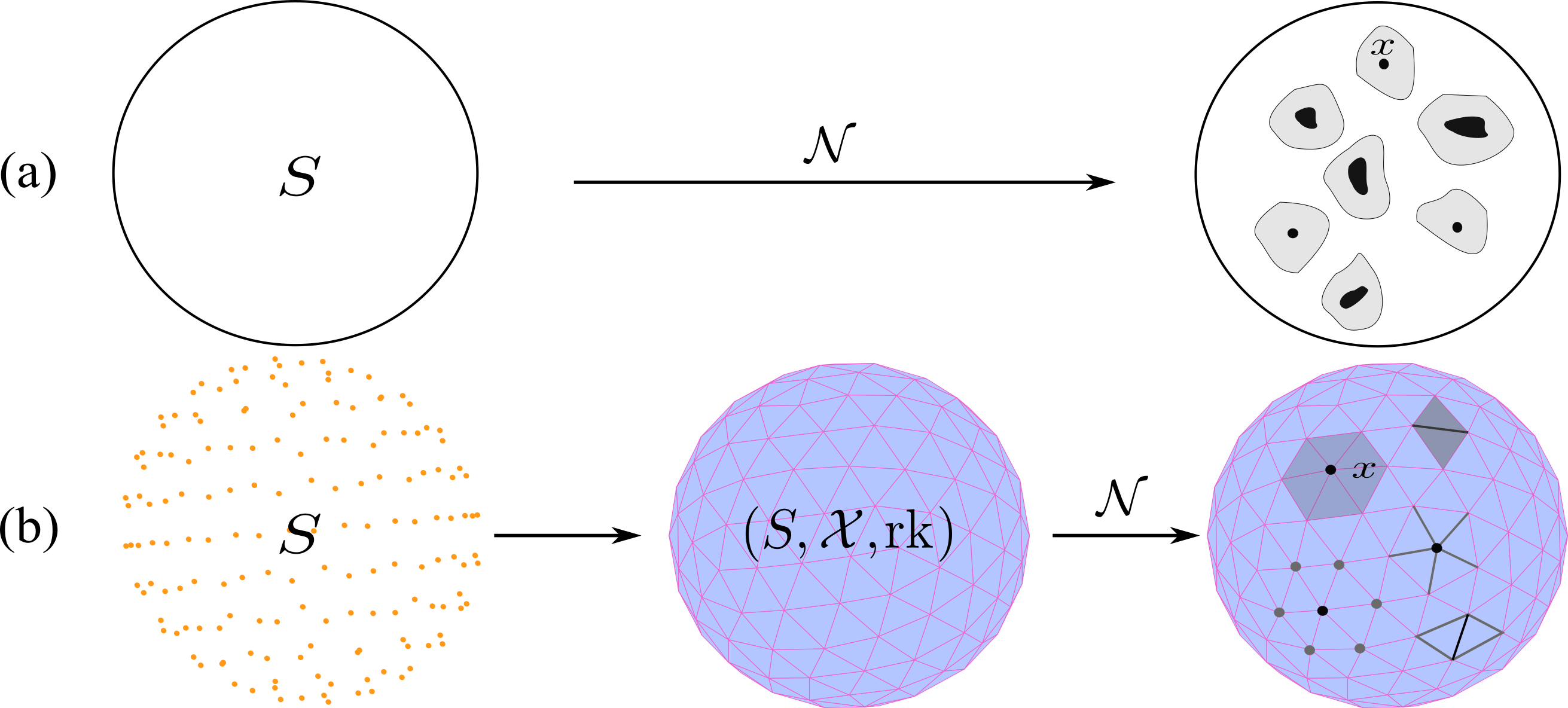
FIGURE 4.5: A visual comparison between neighborhood functions with continuous domains and CC-neighborhood functions. (a): A neighborhood function with a continuous domain \(S\) assigns to \(x\in S\) a set \(\mathcal{N}(x)\) of subsets of \(S\) that are in the local vicinity of \(x\). (b): Similarly, a CC-neighborhood function on a CC \((S,\mathcal{X}, \mbox{rk})\) assigns to \(x\in S\) a set \(\mathcal{N}(x)\) of subsets of \(\mathcal{X}\) that are in the local vicinity of \(x\).
Neighborhood matrix induced by a neighborhood function. For the purposes of computation, it is convenient to represent neighborhood functions as matrices. Incidence, adjacency, and coadjacency matrices are well-known examples of matrices that encode respective neighborhood functions. In Definition 4.5, we introduce a generalization of these matrices called the `neighborhood matrix’. In this definition and henceforth, we denote the cardinality of a set \(S\) by \(|S|\).
Definition 4.5 (Neighborhood matrix) Let \(\mathcal{N}\) be a neighborhood function defined on a CC \(\mathcal{X}\). Moreover, let \(\mathcal{Y}=\{y_1,\ldots,y_n\}\) and \(\mathcal{Z}=\{z_1,\ldots,z_m\}\) be two collections of cells in \(\mathcal{X}\) such that \(\mathcal{N}(y_{i}) \subseteq \mathcal{Z}\) for all \(1\leq i \leq n\). The neighborhood matrix of \(\mathcal{N}\) with respect to \(\mathcal{Y}\) and \(\mathcal{Z}\) is the \(|\mathcal{Z}| \times |\mathcal{Y}|\) binary matrix \(G\) whose \((i,j)\)-th entry \([G]_{ij}\) has value \(1\) if \(z_i \in \mathcal{N}(y_j)\) and \(0\) otherwise.
Remark. In Definition 4.5, \(\mathcal{N}(y_j)\) is stored in the \(j\)-th column of the associated neighborhood matrix \(G\). For this reason, we denote by \(\mathcal{N}_{G}(j)\) the neighborhood function of the cell \(y_j\) when we work with the neighborhood matrix \(G\).
There are many ways to define useful neighborhood functions on a CC. In this work, we constrain ourselves to the most immediate neighborhood functions: the incidence and adjacency neighborhood functions.
4.4.1 Incidence in a CC
We define three notions of incidence to capture different facets of incidence structures of cells in a CC. First, in Definition 4.6, we introduce the down-incidence and up-incidence neighborhood functions to describe the incidence structure of a cell via cells of arbitrary rank. Second, in Definition 4.7, we introduce the \(k\)-down and \(k\)-up incidence neighborhood functions to describe the incidence structure of a cell via cells of a particular rank \(k\). Third, in Definition 4.8, we introduce \((r, k)\)-incidence matrices to describe the incidence structures of cells of particular ranks \(r\) and \(k\). In what follows, we assume that the cells in the set \(\mathcal{X}\) of a CC \((S,\mathcal{X}, \mbox{rk})\) are given a fixed order.
Definition 4.6 (Down/up-incidence neighborhood functions) Let \((S,\mathcal{X}, \mbox{rk})\) be a CC. Two cells \(x, y\in\mathcal{X}\) of the CC are called incident if either \(x \subsetneq y\) or \(y \subsetneq x\). In particular, the down-incidence neighborhood function \(\mathcal{N}_{\searrow}(x)\) of a cell \(x\in\mathcal{X}\) is defined to be the set \(\{ y\in \mathcal{X} \mid y \subsetneq x\}\), while the up-incidence neighborhood function \(\mathcal{N}_{\nearrow}(x)\) of \(x\) is defined to be the set \(\{ y\in \mathcal{X} \mid x \subsetneq y\}\).
Definition 4.7 provides a more granular specification of incidence than Definition 4.6. In particular, Definitions 4.7 and 4.6 describe the incidence structure of a cell with respect to cells of a particular rank or of arbitrary rank, respectively.
Definition 4.7 (k-down/up incidence neighborhood functions) Let \((S,\mathcal{X}, \mbox{rk})\) be a CC. For any \(k\in\mathbb{N}\), the \(k\)-down incidence neighborhood function \(\mathcal{N}_{\searrow,k}(x)\) of a cell \(x\in\mathcal{X}\) is defined to be the set \(\{ y\in \mathcal{X} \mid y \subsetneq x, \mbox{rk}(y)=\mbox{rk}(x)-k \}\). The \(k\)-up incidence neighborhood function \(\mathcal{N}_{\nearrow,k}(x)\) of \(x\) is defined to be the set \(\{ y\in \mathcal{X} \mid y \subsetneq x, \mbox{rk}(y)=\mbox{rk}(x)+k \}\).
Clearly, \(\mathcal{N}_{\searrow}(x)= \bigcup_{k\in \mathbb{N}} \mathcal{N}_{\searrow,k}(x)\) and \(\mathcal{N}_{\nearrow}(x)= \bigcup_{k\in\mathbb{N}} \mathcal{N}_{\nearrow,k}(x)\). Immediate incidence is particularly important. To this end, the set of faces of a cell \(x \in \mathcal{X}\) is defined to be \(\mathcal{N}_{\searrow,1} (x)\), and the set of cofaces of a cell \(x\) is defined to be \(\mathcal{N}_{\nearrow,1} (x)\). An illustration of \(k\)-down and \(k\)-up incidence neighborhood functions is given in Figure 4.6.
Definition 4.8 (Neighborhood matrix) Let \((S,\mathcal{X}, \mbox{rk})\) be a CC. For any \(r,k \in \mathbb{Z}{\ge 0}\) with \(0\leq r<k \leq \dim(\mathcal{X})\), the \((r,k)\)-incidence matrix \(B_{r,k}\) between \(\mathcal{X}^{r}\) and \(\mathcal{X}^{k}\) is defined to be the \(|\mathcal{X}^r| \times |\mathcal{X}^k|\) binary matrix whose \((i, j)\)-th entry \([B_{r,k}]_{ij}\) equals one if \(x^r_i\) is incident to \(x^k_j\) and zero otherwise.
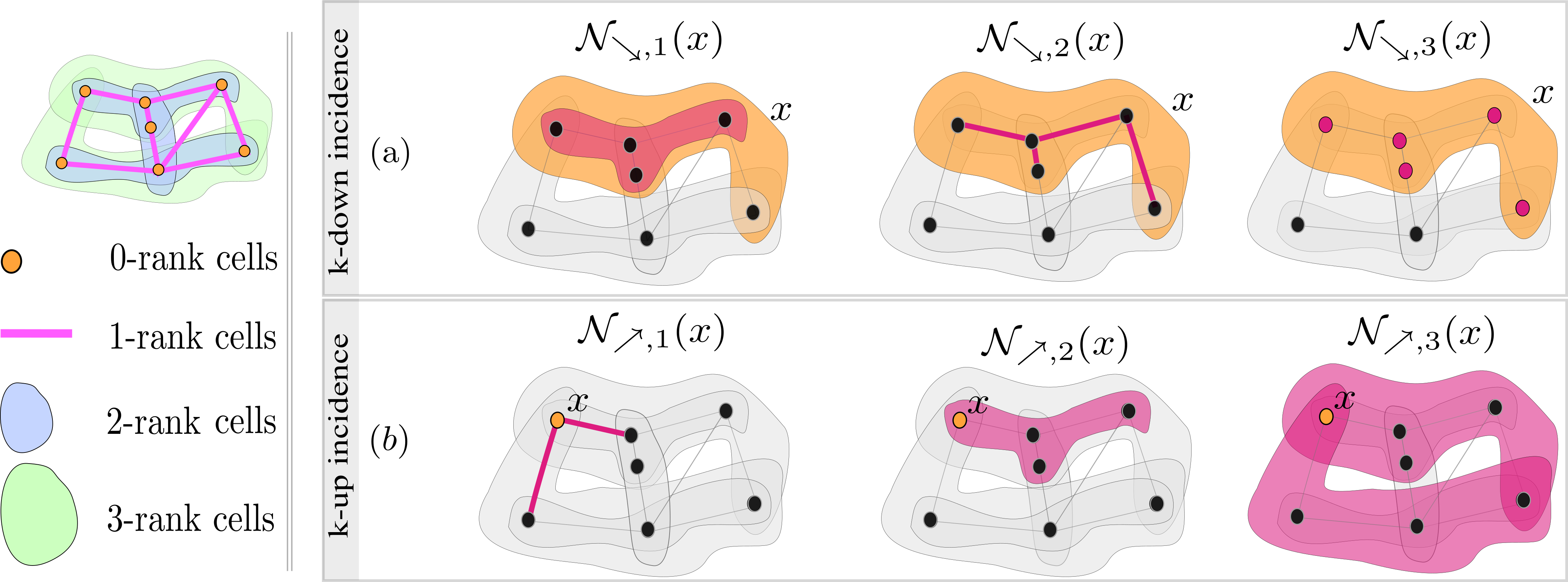
FIGURE 4.6: Illustration of \(k\)-down and \(k\)-up incidence neighborhood functions on a CC of dimension three. (a): Illustration of \(k\)-down incidence neighborhood functions. The target orange cell \(x\) has rank three. From left to right, the red cells represent \(\mathcal{N}_{\searrow,1}(x)\), \(\mathcal{N}_{\searrow,2}(x)\) and \(\mathcal{N}_{\searrow,3}(x)\). (b): Illustration of \(k\)-up incidence neighborhood functions. The target orange cell \(x\) has rank zero. From left to right, the red cells represent \(\mathcal{N}_{\nearrow,1}(x)\), \(\mathcal{N}_{\nearrow,2}(x)\) and \(\mathcal{N}_{\nearrow,3}(x)\).
The incidence matrices \(B_{r,k}\) of Definition 4.8 determine a neighborhood function on the underlying CC. Neighborhood functions induced by incidence matrices are utilized to construct a higher-order message passing scheme on CCs, as described in Chapter 5.
4.4.2 Adjacency in a CC
CCs admit incidence as well as other neighborhood functions. For instance, for a CC that is reduced to a graph, a more natural neighborhood function is based on the notion of adjacency relation. Incidence defines relations among cells of different ranks, while adjacency defines relations among cells of similar ranks. Definitions 4.9, 4.10 and 4.11/4.12 introduce the (co)adjacency analogues of the respective incidence-related Definitions 4.6, 4.7, and 4.8.
Definition 4.9 ((Co)adjacency neighborhood functions) Let \((S,\mathcal{X}, \mbox{rk})\) be a CC. The adjacency neighborhood function \(\mathcal{N}_{a}(x)\) of a cell \(x\in \mathcal{X}\) is defined to be the set \[\begin{equation*} \{ y \in \mathcal{X} \mid \mbox{rk}(y)=\mbox{rk}(x), \exists z \in \mathcal{X} \text{ with } \mbox{rk}(z)>\mbox{rk}(x) \text{ such that } x,y\subsetneq z\}. \end{equation*}\] The coadjacency neighborhood function \(\mathcal{N}_{co}(x)\) of \(x\) is defined to be the set \[\begin{equation*} \{ y \in \mathcal{X} \mid \mbox{rk}(y)=\mbox{rk}(x), \exists z \in \mathcal{X} \text{ with } \mbox{rk}(z)<\mbox{rk}(x) \text{ such that } z\subsetneq y\text{ and }z\subsetneq x \}. \end{equation*}\] A cell \(z\) satisfying the conditions of either \(\mathcal{N}_{a}(x)\) or \(\mathcal{N}_{co}(x)\) is called a bridge cell.
Definition 4.10 (k-(co)adjacency neighborhood functions) Let \((S, \mathcal{X}, \mbox{rk})\) be a CC. For any \(k\in\mathbb{N}\), the \(k\)-adjacency neighborhood function \(\mathcal{N}_{a,k}(x)\) of a cell \(x \in \mathcal{X}\) is defined to be the set \[\begin{equation*} \{ y \in \mathcal{X} \mid \mbox{rk}(y)=\mbox{rk}(x), \exists z \in \mathcal{X} \text{ with } \mbox{rk}(z)=\mbox{rk}(x)+k \text{ such that } x,y\subsetneq z \}. \end{equation*}\] The \(k\)-coadjacency neighborhood function \(\mathcal{N}_{co,k}(x)\) of \(x\) is defined to be the set \[\begin{equation*} \{ y \in \mathcal{X} \mid \mbox{rk}(y)=\mbox{rk}(x), \exists z \in \mathcal{X} \text{ with } \mbox{rk}(z)=\mbox{rk}(x)-k \text{ such that } z\subsetneq y\text{ and }z\subsetneq x \}. \end{equation*}\]
Definition 4.11 (Adjacency matrix) For any \(r\in\mathbb{Z}_{\ge 0}\) and \(k\in \mathbb{Z}_{>0}\) with \(0\leq r<r+k \leq \dim(\mathcal{X})\), the \((r,k)\)-adjacency matrix \(A_{r,k}\) among the cells of \(\mathcal{X}^{r}\) with respect to the cells of \(\mathcal{X}^{k}\) is defined to be the \(|\mathcal{X}^r| \times |\mathcal{X}^r|\) binary matrix whose \((i, j)\)-th entry \([A_{r,k}]_{ij}\) equals one if \(x^r_i\) is \(k\)-adjacent to \(x^r_j\) and zero otherwise.
Definition 4.12 (Coadjacency matrix) For any \(r\in \mathbb{Z}_{\ge 0}\) and \(k\in\mathbb{N}\) with \(0\leq r-k<r \leq \dim(\mathcal{X})\), the \((r,k)\)-coadjacency matrix \(coA_{r,k}\) among the cells of \(\mathcal{X}^{r}\) with respect to the cells of \(\mathcal{X}^{k}\) is defined to be the \(|\mathcal{X}^r| \times |\mathcal{X}^r|\) binary matrix whose \((i, j)\)-th entry \([coA_{r,k}]_{ij}\) has value \(1\) if \(x^r_i\) is \(k\)-coadjacent to \(x^r_j\) and \(0\) otherwise.
Clearly, \(\mathcal{N}_{a}(x)= \cup_{k\in\mathbb{N}} \mathcal{N}_{a,k}(x)\) and \(\mathcal{N}_{co}(x)= \cup_{k\in\mathbb{N}} \mathcal{N}_{co,k}(x)\). An illustration of \(k\)-adjacency and \(k\)-coadjacency neighborhood functions is given in Figure 4.7.
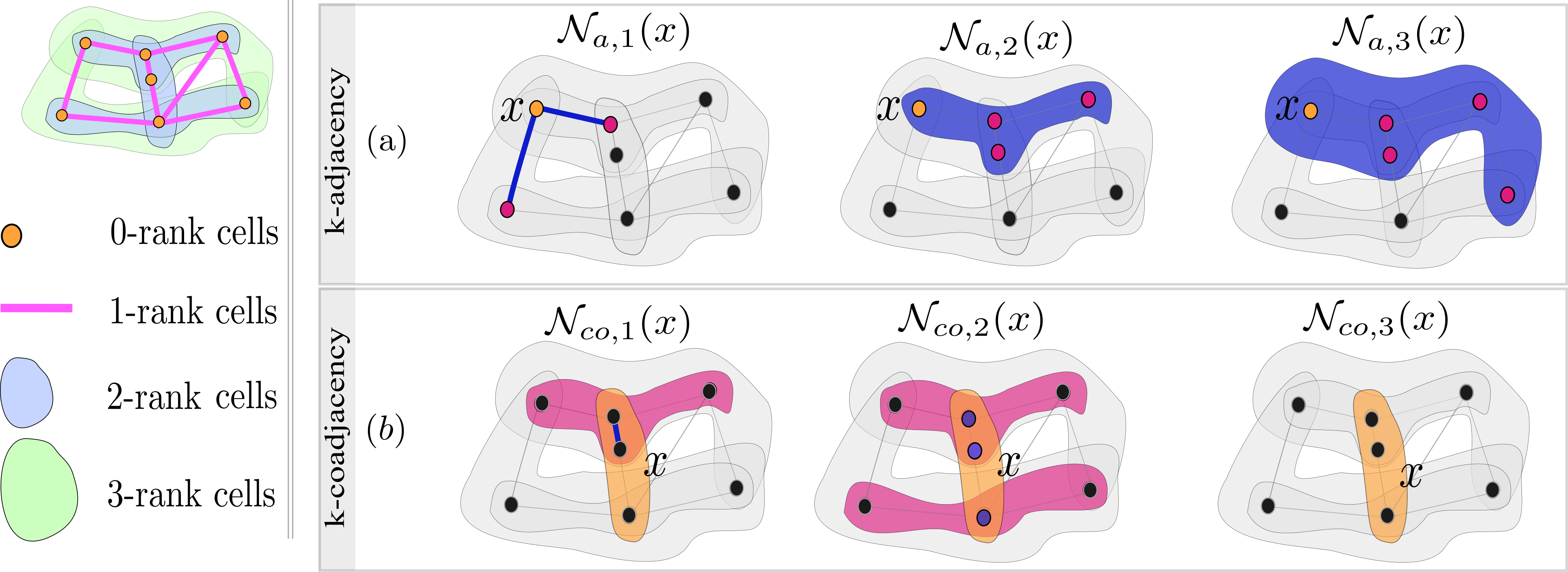
FIGURE 4.7: Illustration of \(k\)-(co)adjacency neighborhood functions on a CC of dimension three. (a): Illustration of \(k\)-adjacency neighborhood functions. The target orange cell \(x\) has rank zero. From left to right, the red cells represent \(\mathcal{N}_{a,1}(x)\), \(\mathcal{N}_{a,2}(x)\) and \(\mathcal{N}_{a,3}(x)\). (b): Illustration of \(k\)-coadjacency neighborhood functions. The target orange cell \(x\) has rank two. From left to right, the red cells represent \(\mathcal{N}_{co,1}(x)\), \(\mathcal{N}_{co,2}(x)\) and \(\mathcal{N}_{co,3}(x)\).
4.5 Data on CCs
As we are interested in processing the data defined over a CC \((S,\mathcal{X},\mbox{rk})\), we introduce \(k\)-cochain spaces, \(k\)-cochains and cochain maps.
Definition 4.13 (k-cochain spaces) Let \(\mathcal{C}^k(\mathcal{X},\mathbb{R}^d )\) be the \(\mathbb{R}\)-vector space of functions \(\mathbf{H}_k\colon\mathcal{X}^k\to \mathbb{R}^d\) for a rank \(k \in \mathbb{Z}_{\ge 0}\) and dimension \(d\). \(d\) is called the data dimension. \(\mathcal{C}^k(\mathcal{X},\mathbb{R}^d)\) is called the \(k\)-cochain space. Elements \(\mathbf{H}_k\) in \(\mathcal{C}^k(\mathcal{X},\mathbb{R}^d)\) are called \(k\)-cochains or \(k\)-signals.
We use the notation \(\mathcal{C}^k(\mathcal{X})\) or \(\mathcal{C}^k\) when the underlying CC is clear. Moreover, we say that a \(k\)-cochain space \(\mathcal{C}^k(\mathcal{X})\) is defined on \(\mathcal{X}\). Intuitively, a \(k\)-cochain can be interpreted as a signal defined on the \(k\)-cells of \(\mathcal{X}\) (Grady and Polimeni 2010). Figure 4.8(a) shows an example of a cochain supported on 0, 1, and 2-rank cells of a simplicial complex.
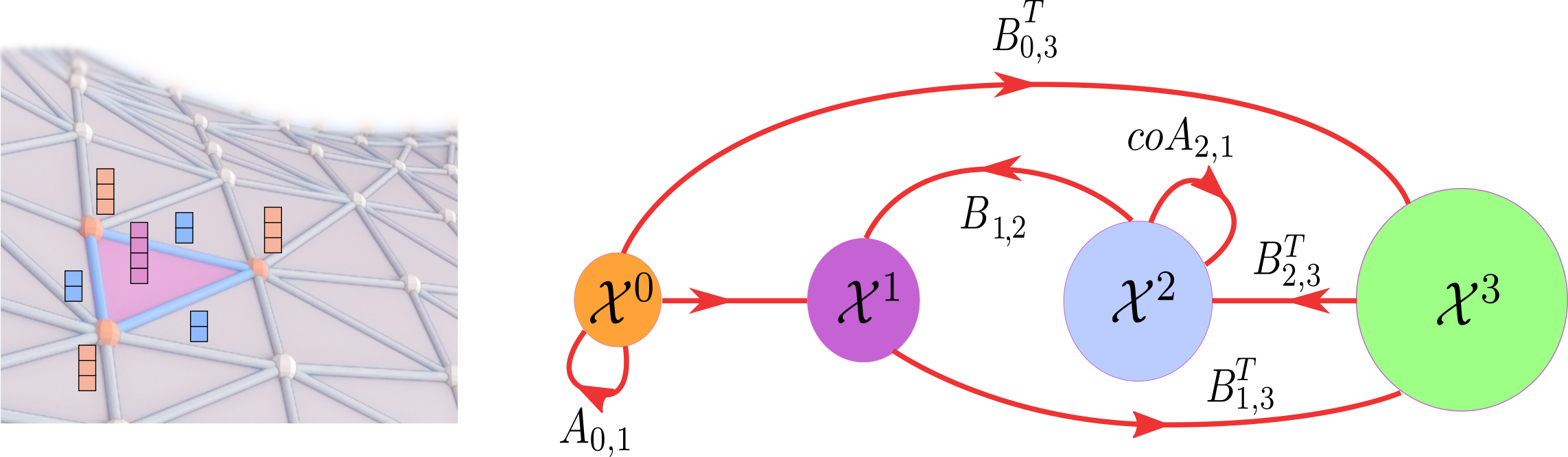
FIGURE 4.8: Examples of \(k\)-cochains (left) and cochain maps (right) supported on a CC of dimension four. Left: a \(k\)-cochain can be interpreted as a signal or a feature vector defined on the \(k\)-cells. In the figure, a 3-dimensional cochain is attached to the vertices, 2-dimensional cochains are attached to the 1-cells, and 4-dimensional cochains to the 2-cells. Right: each of \(coA_{r,k}\) and \(A_{r,k}\) defines a cochain map between cochain spaces of equal dimension, whereas each \(B_{r,k}\) defines a cochain map between cochain spaces of different dimensions.
When \(\mathcal{X}\) is a graph, \(0\)-cochains correspond to graph signals (Ortega et al. 2018). Ordering the cells in \(\mathcal{X}^k\), we canonically identify \(\mathcal{C}^k(\mathcal{X},\mathbb{R}^d )\) with the Euclidean vector space \(\mathbb{R}^{ |\mathcal{X}^k| \times d}\) and explicitly write \(\mathbf{H}_k\) as the vector \([ \mathbf{h}_{x^k_1},\ldots,\mathbf{h}_{x^k_{|\mathcal{X}^k|} }]\), where \(\mathbf{h}_{x^k_j} \in \mathbb{R}^d\) is a feature vector associated with the cell \(x^k_j\). The notation \(\mathbf{H}_{k,j}\) refers to the feature vector \(\mathbf{h}_{x^k_j}\) to avoid explicit reference to cell \(x^k_j\). We also work with maps between cochain spaces, which we call cochain maps.
Definition 4.14 (Cochain maps) For \(r< k\), an incidence matrix \(B_{r,k}\) induces a map \[\begin{align*} B_{r,k}\colon \mathcal{C}^k(\mathcal{X}) &\to \mathcal{C}^r(\mathcal{X}),\\ \mathbf{H}_k &\to B_{r,k}(\mathbf{H}_k), \end{align*}\] where \(B_{r,k}(\mathbf{H}_k)\) denotes the usual product \(B_{r,k} \mathbf{H}_k\) of matrix \(B_{r,k}\) with vector \(\mathbf{H}_k\). Similarly, an \((r,k)\)-adjacency matrix \(A_{r,k}\) induces a map \[\begin{align*} A_{r,k}\colon \mathcal{C}^r(\mathcal{X}) &\to \mathcal{C}^r(\mathcal{X}),\\ \mathbf{H}_r &\to A_{r,k}(\mathbf{H}_r). \end{align*}\] These two types of maps between cochain spaces are called cochain maps.
Cochain maps serve as operators that ‘shuffle’ and ‘redistribute’ the data on the underlying CC. In the context of TDL, cochain maps are the main tools for defining higher-order message passing (Section 6.1) as well as (un)pooling operations (Section 7.1). Each adjacency matrix \(A_{r,k}\) or coadjacency matrix \(coA_{r,k}\) defines a cochain map between cochain spaces of equal dimension, while each incidence matrix \(B_{r,k}\) defines a cochain map between different dimensions. Figure 4.8(b) shows examples of cochain maps on a CC of dimension 4.