Chapter 5 Combinatorial complex neural networks
The modelling flexibility of CCs enables the exploration and analysis of a wide spectrum of CC-based neural network architectures. A CC-based neural network can exploit all neighborhood matrices or a subset of them, thus accounting for multi-way interactions among various cells in the CC to solve a learning task. In this section, we introduce the blueprint for TDL by developing the general principles of CC-based TDL models. We utilize our TDL blueprint framework for examining current approaches and offer directives for designing novel models.
The learning tasks in TDL can be broadly classified into three categories: cell classification, complex classification, and cell prediction. See Figure 5.1. Our numerical experiments in Chapter 9 provide examples on cell and complex classification. In more detail, the learning tasks of the three categories are the following:
- Cell classification: the goal is to predict targets for each cell in a complex. To accomplish this, we can utilize a TDL classifier that takes into account the topological neighbors of the target cell and their associated features. An example of cell classification is triangular mesh segmentation, in which the task is to predict the class of each face or edge in a given mesh.
- Complex classification: the aim is to predict targets for an entire complex. To achieve this, we can reduce the topology of the complex into a common representation using higher-order cells, such as pooling, and then learn a TDL classifier over the resulting flat vector. An example of complex classification is class prediction for each input mesh.
- Cell prediction: the objective is to predict properties of cell-cell interactions in a complex, and, in some cases, to predict whether a cell exists in the complex. This can be achieved by utilizing the topology and associated features of the cells. A relevant example is the prediction of linkages among entities in hyperedges of a hypergraph.
FIGURE 5.1: Learning on topological spaces can be broadly classified in three main tasks. (1) Cell classification: this task predicts targets for individual cells within a complex. An example of this tasks is mesh segmentation where the topological neural network outputs a segmentation label for every face in the input mesh. (2) Complex classification: predicting targets for entire complexes involves reducing topology into a common representation. An example of this task is class prediction for input meshes. (3) Cell prediction: forecasting properties of cell-cell interactions, sometimes including predicting cell existence, by leveraging topology of the underlying complex and associated features. An example of this task is predicting linkages in hypergraph hyperedges.
Figure 5.2 outlines our general setup for TDL. Initially, a higher-order domain, represented by a CC, is constructed on a set \(S\). A set of neighborhood functions defined on the domain is then selected. The neighborhood functions are usually selected based on the learning problem at hand and they are used to build a topological neural network. To develop our general TDL framework, we introduce combinatorial complex neural networks (CCNNs), an abstract class of neural networks supported on CCs that effectively captures the pipeline of Figure 5.2. CCNNs can be thought of as a template that generalizes many popular architectures, such as convolutional and attention-based neural networks. The abstraction of CCNNs offers many advantages. First, any result that holds for CCNNs is immediately applicable to any particular instance of CCNN architecture. Indeed, the theoretical analysis and results in this paper are applicable to any CC-based neural network as long as it satisfies the CCNN definition. Second, working with a particular parametrization might be cumbersome if the neural network has a complicated architecture. In Section 5.1, we elaborate on the intricate architectures of parameterized TDL models. The more abstract high-level representation of CCNNs simplifies the notation and the general purpose of the learning process, thereby making TDL modelling more intuitive to handle.
FIGURE 5.2: A TDL blueprint. (a): A set of abstract entities. (b): A CC \((S, \mathcal{X}, \mbox{rk})\) is defined on \(S\). (c): For an element \(x \in \mathcal{X}\), we select a collection of neighborhood functions defined on the CC. (d): We build a neural network on the CC using the neighborhood functions selected in (c). The neural network exploits the neighborhood functions selected in (c) to update the data supported on \(x\).
Definition 5.1 (Combinatorial complex neural networks) Let \(\mathcal{X}\) be a CC. Let \(\mathcal{C}^{i_1}\times\mathcal{C}^{i_2}\times \ldots \times \mathcal{C}^{i_m}\) and \(\mathcal{C}^{j_1}\times\mathcal{C}^{j_2}\times \ldots \times \mathcal{C}^{j_n}\) be a Cartesian product of \(m\) and \(n\) cochain spaces defined on \(\mathcal{X}\). A combinatorial complex neural network (CCNN) is a function of the form \[\begin{equation*} \mbox{CCNN}: \mathcal{C}^{i_1}\times\mathcal{C}^{i_2}\times \ldots \times \mathcal{C}^{i_m} \longrightarrow \mathcal{C}^{j_1}\times\mathcal{C}^{j_2}\times \ldots \times \mathcal{C}^{j_n}. \end{equation*}\]
Intuitively, a CCNN takes a vector of cochains \((\mathbf{H}_{i_1},\ldots, \mathbf{H}_{i_m})\) as input and returns a vector of cochains \((\mathbf{K}_{j_1},\ldots, \mathbf{K}_{j_n})\) as output. In Section 5.1, we show how neighborhood functions play a central role in the construction of a general CCNN. Definition 5.1 does not show how a CCNN can be computed in general. Chapters 6 and 7 formalize the computational workflow in CCNNs.
5.1 Building CCNNs: tensor diagrams
Unlike graphs that involve vertex or edge signals, higher-order networks entail a higher number of signals (see Figure 4.8). Thus, constructing a CCNN requires building a non-trivial amount of interacting sub-neural networks. Due to the potentially large number of cochains procssed via a CCNN, we introduce tensor diagrams, a diagrammatic notation for that describes a generic computational model supported on a topological domain and describing the flow of various signals supported and processed on this domain.
Remark. Diagrammatic notation is common in the geometric topology literature (Hatcher 2005; Turaev 2016), and it is typically used to construct functions built from simpler building blocks. See Appendix C for further discussion. See also (T. Mitchell Roddenberry, Glaze, and Segarra 2021) for related constructions on simplicial neural networks.
Definition 5.2 (Tensor diagram) A tensor diagram represents a CCNN via a directed graph. The signal on a tensor diagram flows from the source nodes to the target nodes. The source and target nodes correspond to the domain and codomain of the CCNN.
Figure 5.3 depicts an example of a tensor diagram. On the left, a CC of dimension three is shown. Consider a 0-cochain \(\mathcal{C}^0\), a 1-cochain \(\mathcal{C}^1\) and a 2-cochain \(\mathcal{C}^2\). The middle figure displays a CCNN that maps a cochain vector in \(\mathcal{C}^0 \times \mathcal{C}^1\times \mathcal{C}^2\) to a cochain vector in \(\mathcal{C}^0\times\mathcal{C}^1 \times \mathcal{C}^2\). On the right, a tensor diagram representation of the CCNN is shown. We label each edge on the tensor diagram by a cochain map or by its matrix representation. The edge labels on the tensor diagram of Figure 5.3 are \(A_{0,1}, B_{0,1}^{T}, A_{1,1}, B_{1,2}\) and \(coA_{2,1}\). Thus, the tensor diagram specifies the flow of cochains on the CC.
FIGURE 5.3: A tensor diagram is a diagrammatic representation of a CCNN that captures the flow of signals on the CCNN.
The labels on the arrows of a tensor diagram form a sequence \(\mathbf{G}= (G_i)_{i=1}^l\) of cochain maps defined on the underlying CC. In Figure 5.3 for example, \(\mathbf{G}=(G_i)_{i=1}^5 = (A_{0,1}, B_{0,1}^{T}, A_{1,1}, B_{1,2}, coA_{2,1})\). When a tensor diagram is used to represent a CCNN, we use the notation \(\mbox{CCNN}_{\mathbf{G}}\) for the tensor diagram and for its corresponding CCNN. The cochain maps \((G_i)_{i=1}^l\) reflect the structure of the CC and are used to determine the flow of signals on the CC. Any of the neighborhood matrices mentioned in Section 4.4 can be used as cochain maps. The choice of cochain maps depends on the learning task.
Figure 5.4 visualizes additional examples of tensor diagrams. The height of a tensor diagram is the number of edges on a longest path from a source node to a target node. For instance, the heights of the tensor diagrams in Figures 5.4(a) and 5.4(d) are one and two, respectively. The vertical concatenation of two tensor diagrams represents the composition of their corresponding CCNNs. For example, the tensor diagram in Figure 5.4(d) is the vertical concatenation of the tensor diagrams in Figures 5.4(c) and (b).
FIGURE 5.4: Examples of tensor diagrams. (a): Tensor diagram of a \(\mbox{CCNN}_{coA_{1,1}}\colon \mathcal{C}^1 \to \mathcal{C}^1\). (b): Tensor diagram of a \(\mbox{CCNN}_{ \{B_{1,2}, B_{1,2}^T\}} \colon \mathcal{C}^1 \times \mathcal{C}^2 \to \mathcal{C}^1 \times \mathcal{C}^2\). (c): A merge node that merges three cochains. (d): A tensor diagram generated by vertical concatenation of the tensor diagrams in (c) and (b). The edge label \(Id\) denotes the identity matrix.
If a node in a tensor diagram receives one or more signals, we call it a merge node. Mathematically, a merge node is a function \(\mathcal{M}_{G_1,\ldots ,G_m}\colon \mathcal{C}^{i_1}\times\mathcal{C}^{i_2}\times \ldots \times \mathcal{C}^{i_m} \to \mathcal{C}^{j}\) given by \[\begin{equation} (\mathbf{H}_{i_1},\ldots,\mathbf{H}_{i_m}) \xrightarrow[]{\mathcal{M}} \mathbf{K}_{j}= \mathcal{M}_{G_1,\ldots,G_m}(\mathbf{H}_{i_1},\ldots,\mathbf{H}_{i_m}), \tag{5.1} \end{equation}\] where \(G_k \colon C^{i_k}(\mathcal{X})\to C^{j}(\mathcal{X}), k=1,\ldots,m\), are cochain maps. We think of \(\mathcal{M}\) as a message-passing function that takes into account the messages outputted by maps \(G_1,\ldots,G_m\), which collectively act on a cochain vector \((\mathbf{H}_{i_1},\ldots,\mathbf{H}_{i_m})\), to obtain an updated cochain \(\mathbf{K}_{j}\). See Sections 5.2 and 6.2 for more details. Figure 5.4(c) shows a merge node example.
5.2 Push-forward operator and merge node
We introduce the push-forward operation, a computational scheme that enables sending a cochain supported on \(i\)-cells to \(j\)-cells. The push-forward operation is a computational building block used to formalize the definition of the merge nodes given in Equation (5.1), the higher-order message passing introduced in Chapter 6, and the (un)pooling operations introduced in Section 7.
Definition 5.3 (Cochain push-forward) Consider a CC \(\mathcal{X}\), a cochain map \(G\colon\mathcal{C}^i(\mathcal{X})\to \mathcal{C}^j(\mathcal{X})\), and a cochain \(\mathbf{H}_i\) in \(\mathcal{C}^i(\mathcal{X})\). A (cochain) push-forward induced by \(G\) is an operator \(\mathcal{F}_G \colon \mathcal{C}^i(\mathcal{X})\to \mathcal{C}^j(\mathcal{X})\) defined via \[\begin{equation} \mathbf{H}_i \to \mathbf{K}_j=[ \mathbf{k}_{y^j_1},\ldots,\mathbf{k}_{y^j_{|\mathcal{X}^j|} }] = \mathcal{F}_G(\mathbf{H}_i), \end{equation}\] such that for \(k=1,\ldots,|\mathcal{X}^j|\), \[\begin{equation} \mathbf{k}_{y_k^j}= \bigoplus_{x_l^i \in \mathcal{N}_{G^T(y_k^j)}} \alpha_{G} ( \mathbf{ \mathbf{h}_{x_l^i}}), \tag{5.2} \end{equation}\] where \(\bigoplus\) is a permutation-invariant aggregation function and \(\alpha_G\) is a differentiable function.
The operator \(\mathcal{F}_{G}\) pushes forward an \(i\)-cochain \(\mathbf{H}_i\) supported on \(\mathcal{X}^i\) to a \(j\)-cochain \(\mathcal{F}_{G}(\mathbf{H}_i)\) supported on \(\mathcal{X}^j\). For every cell \(y \in \mathcal{X}^j\), Equation (5.2) constructs the vector \(\mathbf{k}_y\) by aggregating all vectors \(\mathbf{h}_x\) attached to the neighbors \(x \in \mathcal{X}^i\) of \(y\) with respect to the neighborhood function \(\mathcal{N}_{G^T}\), and by then applying a differentiable function \(\alpha_G\) on the set of aggregated vectors \(\{ \mathbf{h}_x| x\in \mathcal{N}_{G^T}(y)\}\).
Figure 5.5 visualizes two examples of push-forward operators. Example 5.1 provides a push-forward function induced by an indicence matrix. The push-forward function in Example 5.1 does not contain any parameters, therefore it is not trainable. In Section 5.4, we give examples of parameterized push-forward operations, whose parameters can be learnt.
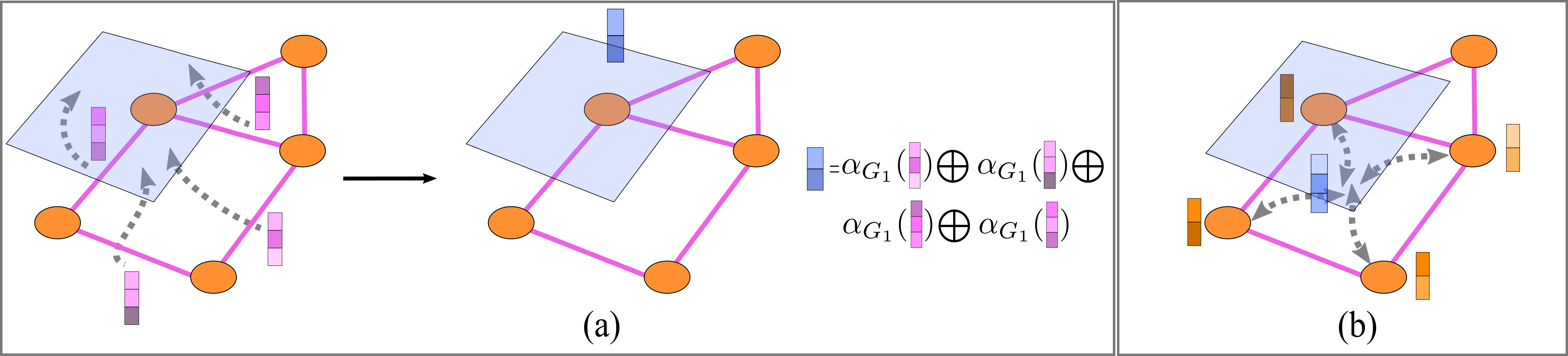
FIGURE 5.5: Examples of push-forward operators. (a): Let \(G_1\colon \mathcal{C}^1\to \mathcal{C}^2\) be a cochain map. A push-forward \(\mathcal{F}_{G_1}\) induced by \(G_1\) takes as input a 1-cochain \(\textbf{H}_{1}\) defined on the edges of the underlying CC \(\mathcal{X}\) and ‘pushes-forward’ this cochain to a 2-cochain \(\mathbf{K}_2\) defined on \(\mathcal{X}^2\). The cochain \(\mathbf{K}_2\) is formed by aggregating the information in \(\mathbf{H}_1\) using the neighborhood function \(\mathcal{N}_{G_1^T}\). In this case, the neighbors of the 2-rank (blue) cell with respect to \(G_1\) are the four (pink) edges on the boundary of this cell. (b): Similarly, \(G_2\colon \mathcal{C}^0\to \mathcal{C}^2\) induces a push-forward map \(\mathcal{F}_{G_2}\colon \mathcal{C}^0\to \mathcal{C}^2\) that sends a 0-cochain \(\mathbf{H}_0\) to a 2-cochain \(\mathbf{K}_2\). The cochain \(\mathbf{K}_2\) is defined by aggregating the information in \(\mathbf{H}_0\) using the neighborhood function \(\mathcal{N}_{G_2^T}\).
Example 5.1 (Push-forward of a CC of dimension two) Consider a CC \(\mathcal{X}\) of dimension 2. Let \(B_{0,2}\colon \mathcal{C}^2 (\mathcal{X})\to \mathcal{C}^0 (\mathcal{X})\) be an incidence matrix. The function \(\mathcal{F}^{m}_{B_{0,2}}\colon\mathcal{C}^2 (\mathcal{X})\to \mathcal{C}^0 (\mathcal{X})\) defined by \(\mathcal{F}^{m}_{B_{0,2}}(\mathbf{H_{2}})= B_{0,2} (\mathbf{H}_{2})\) is a push-forward induced by \(B_{0,2}\). \(\mathcal{F}^{m}_{B_{0,2}}\) pushes forward the cochain \(\mathbf{H}_{2}\in \mathcal{C}^2\) to cochain \(B_{0,2} (\mathbf{H}_{2}) \in \mathcal{C}^0\).
In Definition 5.4, we formulate the notion of merge node using push-forward operators. Figure 5.6 visualizes Definition @ref(def:exact_definition-merge-node) of merge node via a tensor diagram.
Definition 5.4 (Merge node) Let \(\mathcal{X}\) be a CC. Moreover, let \(G_1\colon\mathcal{C}^{i_1}(\mathcal{X})\to\mathcal{C}^j(\mathcal{X})\) and \(G_2\colon\mathcal{C}^{i_2}(\mathcal{X})\to\mathcal{C}^j(\mathcal{X})\) be two cochain maps. Given a cochain vector \((\mathbf{H}_{i_1},\mathbf{H}_{i_2}) \in \mathcal{C}^{i_1}\times \mathcal{C}^{i_2}\), a merge node \(\mathcal{M}_{G_1,G_2}\colon\mathcal{C}^{i_1} \times \mathcal{C}^{i_2} \to \mathcal{C}^j\) is defined as \[\begin{equation} \mathcal{M}_{G_1,G_2}(\mathbf{H}_{i_1},\mathbf{H}_{i_2})= \beta\left( \mathcal{F}_{G_1}(\mathbf{H}_{i_1}) \bigotimes \mathcal{F}_{G_2}(\mathbf{H}_{i_2}) \right), \end{equation}\] where \(\bigotimes \colon \mathcal{C}^j \times \mathcal{C}^j \to \mathcal{C}^j\) is an aggregation function, \(\mathcal{F}_{G_1}\) and \(\mathcal{F}_{G_2}\) are push-forward operators induced by \(G_1\) and \(G_2\), and \(\beta\) is an activation function.
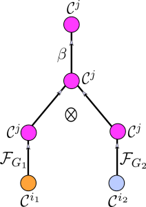
FIGURE 5.6: Visualization of the definition of merge node.
5.3 The main three tensor operations
Any tensor diagram representation of a CCNN can be built from two elementary operations: the push-forward operator and the merge node. In practice, it is convenient to introduce other operations that facilitate building involved neural network architectures more effectively. For example, one useful operation is the dual operation of the merge node, which we call the split node.
Definition 5.5 (Split node) Let \(\mathcal{X}\) be a CC. Moreover, let \(G_1\colon\mathcal{C}^{j}(\mathcal{X})\to\mathcal{C}^{i_1}(\mathcal{X})\) and \(G_2\colon\mathcal{C}^{j}(\mathcal{X})\to\mathcal{C}^{i_2}(\mathcal{X})\) be two cochain maps. Given a cochain \(\mathbf{H}_{j} \in \mathcal{C}^{j}\), a split node \(\mathcal{S}_{G_1,G_2}\colon\mathcal{C}^j \to \mathcal{C}^{i_1} \times \mathcal{C}^{i_2}\) is defined as \[\begin{equation} \mathcal{S}_{G_1,G_2}(\mathbf{H}_{j})= \left( \beta_1(\mathcal{F}_{G_1}(\mathbf{H}_{j})) , \beta_2(\mathcal{F}_{G_2}(\mathbf{H}_{j})) \right), \end{equation}\] where \(\mathcal{F}_{G_i}\) is a push-forward operator induced by \(G_i\), and \(\beta_i\) is an activation function for \(i=1, 2\).
While it is clear from Definition 5.5 that split nodes are simply tuples of push-forward operations, using split nodes allows us to build neural networks more effectively and intuitively. Definition 5.6 puts forward a set of elementary tensor operations, including split nodes, to facilitate the formulation of CCNNs in terms of tensor diagrams.
Definition 5.6 (Elementary tensor operations) We refer collectively to push-forward operations, merge nodes and split nodes as elementary tensor operations.
Figure 5.7 displays tensor diagrams of elementary tensor operations, and Figure 5.8 exemplifies how existing topological neural networks are expressed via tensor diagrams based on elementary tensor operations. For example, the simplicial complex net (SCoNe), a Hodge decomposition-based neural network proposed by (T. Mitchell Roddenberry, Glaze, and Segarra 2021), can be effectively realized in terms of split and merge nodes, as shown in Figure 5.8(a).
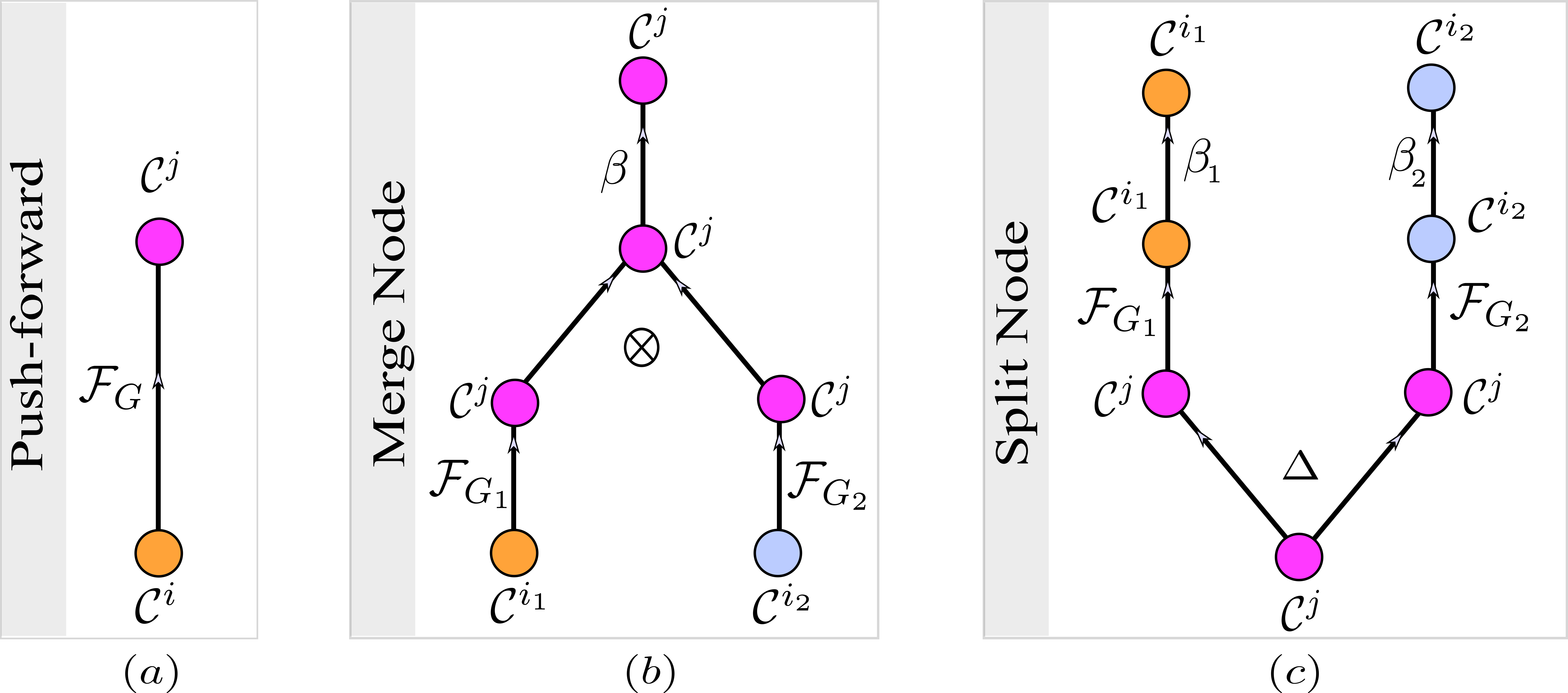
FIGURE 5.7: Tensor diagrams of the elementary tensor operations, namely of push-forward operations, merge nodes and split nodes. These three elementary tensor operations are building blocks for constructing tensor diagrams of general CCNNs. A general tensor diagram can be formed using compositions and horizontal concatenations of the three elementary tensor operations. (a): A tensor diagram of a push-forward operation induced by a cochain map \(G\colon\mathcal{C}^i \to \mathcal{C}^j\). (b): A merge node induced by two cochain maps \(G_1\colon\mathcal{C}^{i_1} \to \mathcal{C}^j\) and \(G_2\colon\mathcal{C}^{i_2} \to \mathcal{C}^j\). (c): A split node induced by two cochain maps \(G_1\colon\mathcal{C}^{j}\to\mathcal{C}^{i_1}\) and \(G_2\colon\mathcal{C}^{j}\to\mathcal{C}^{i_2}\). In this illustration, the function \(\Delta \colon \mathcal{C}^{j}\to \mathcal{C}^{j}\times \mathcal{C}^{j}\) is defined as \(\Delta(\mathbf{H}_j)= (\mathbf{H}_j,\mathbf{H}_j)\).
![Examples of existing neural networks that can be realized in terms of the three elementary tensor operations. Edge labels are dropped to simplify exposition. (a): The simplicial complex net (SCoNe), proposed by [@roddenberry2021principled], can be realized as a composition of a split node that splits an input 1-cochain to three cochains of dimensions zero, one, and two, followed by a merge node that merges these cochains into a 1-cochain. (b): The simplicial neural network (SCN), proposed by [@ebli2020simplicial], can be realized in terms of push-forward operations. (c)--(e): Examples of cell complex neural networks (CXNs); see [@hajijcell]. Note that (e) can be realized in terms of a single merge node that merges the 0 and 2-cochains to a 1-cochain as well as a single split node that splits the 1-cochain to 0- and 2-cochains.](figures/prior_work.png)
FIGURE 5.8: Examples of existing neural networks that can be realized in terms of the three elementary tensor operations. Edge labels are dropped to simplify exposition. (a): The simplicial complex net (SCoNe), proposed by (T. Mitchell Roddenberry, Glaze, and Segarra 2021), can be realized as a composition of a split node that splits an input 1-cochain to three cochains of dimensions zero, one, and two, followed by a merge node that merges these cochains into a 1-cochain. (b): The simplicial neural network (SCN), proposed by (Ebli, Defferrard, and Spreemann 2020), can be realized in terms of push-forward operations. (c)–(e): Examples of cell complex neural networks (CXNs); see (Hajij, Istvan, and Zamzmi 2020). Note that (e) can be realized in terms of a single merge node that merges the 0 and 2-cochains to a 1-cochain as well as a single split node that splits the 1-cochain to 0- and 2-cochains.
Remark. The elementary tensor operations constitute the only framework needed to define any parameterized topological neural network. Indeed, since tensor diagrams can be built via the three elementary tensor operations, then it suffices to define the push-forward and the merge operators in order to fully define a parameterized class of CCNNs (recall that the split node is completely determined by the push-forward operator). In Sections 5.4 and 5.5, we build two parameterized classes of CCNNs: the convolutional and attention classes. In both cases, we only define their corresponding parameterized elementary tensor operations. Beyond convolutional and attention versions of CCNNs, the three elementary tensor operations allow us to build arbitrary parameterized tensor diagrams, therefore providing scope to discover novel topological neural network architectures on which our theory remains applicable.
An alternative way of constructing CCNNs draws ideas from topological quantum field theory (TQFT). In Appendix C, we briefly discuss this relationship in more depth.
5.4 Definition of combinatorial complex convolutional networks
One of the fundamental computational requirements for deep learning on higher-order domains is the ability to define and compute convolutional operations. Here, we introduce CCNNs equipped with convolutional operators, which we call combinatorial complex convolutional neural networks (CCCNNs). In particular, we put forward two convolutional operators for CCCNNs: CC-convolutional push-forward operators and CC-convolutional merge nodes.
We demonstrate how CCCNNs can be introduced from the two basic blocks: the push-forward and the merge operations which have been defined abstractly in Section 5.2. In its simplest form, a CC-convolutional push-forward, as conceived in Definition 5.7, is a generalization of the convolutional graph neural network introduced in (Kipf and Welling 2016).
Definition 5.7 (CC-convolutional push-forward) Consider a CC \(\mathcal{X}\), a cochain map \(G\colon \mathcal{C}^i (\mathcal{X}) \to \mathcal{C}^j(\mathcal{X})\), and a cochain \(\mathbf{H}_i \in C^i(\mathcal{X}, \mathbb{R}^{{s}_{in}})\). A CC-convolutional push-forward is a cochain map \(\mathcal{F}^{conv}_{G;W} \colon C^i(\mathcal{X}, \mathbb{R}^{{s}_{in}}) \to C^j(\mathcal{X}, \mathbb{R}^{{t}_{out}})\) defined as \[\begin{equation} \mathbf{H}_i \to \mathbf{K}_j= G \mathbf{H}_i W , \tag{5.3} \end{equation}\] where \(W \in \mathbb{R}^{d_{s_{in}}\times d_{s_{out}}}\) are trainable parameters.
Having defined the CC-convolutional push-forward, the CC-convolutional merge node (Definition 5.8) is a straightforward application of Definition 5.4. Variants of Definition 5.8 have appeared in recent works on higher-order networks (Bunch et al. 2020; Ebli, Defferrard, and Spreemann 2020; Hajij, Istvan, and Zamzmi 2020; Schaub et al. 2020, 2021; T. Mitchell Roddenberry, Glaze, and Segarra 2021; Calmon, Schaub, and Bianconi 2022; Hajij, Zamzmi, et al. 2022; T. Mitchell Roddenberry, Schaub, and Hajij 2022; Yang and Isufi 2023).
Definition 5.8 (CC-convolutional merge node) Let a \(\mathcal{X}\) be a CC. Moreover, let \(G_1\colon\mathcal{C}^{i_1}(\mathcal{X}) \to\mathcal{C}^j(\mathcal{X})\) and \(G_2\colon\mathcal{C}^{i_2}(\mathcal{X})\to\mathcal{C}^j(\mathcal{X})\) be two cochain maps. Given a cochain vector \((\mathbf{H}_{i_1},\mathbf{H}_{i_2}) \in \mathcal{C}^{i_1}\times \mathcal{C}^{i_2}\), a CC-convolutional merge node \(\mathcal{M}^{conv}_{\mathbf{G};\mathbf{W}} \colon\mathcal{C}^{i_1} \times \mathcal{C}^{i_2} \to \mathcal{C}^j\) is defined as \[\begin{equation} \begin{aligned} \mathcal{M}^{conv}_{\mathbf{G};\mathbf{W}} (\mathbf{H}_{i_1},\mathbf{H}_{i_2}) &= \beta\left( \mathcal{F}^{conv}_{G_1;W_1}(\mathbf{H}_{i_1}) + \mathcal{F}^{conv}_{G_2;W_2}(\mathbf{H}_{i_2}) \right)\\ &= \beta ( G_1 \mathbf{H}_{i_1} W_1 + G_2 \mathbf{H}_{i_2} W_2 ),\\ \end{aligned} \end{equation}\] where \(\mathbf{G}=(G_1, G_2)\), \(\mathbf{W}=(W_1, W_2)\) is a tuple of trainable parameters, and \(\beta\) is an activation function.
In practice, the matrix representation of the cochain map \(G\) in Definition 5.7 might require problem-specific normalization during training. For various types of normalization in the context of higher-order convolutional operators, we refer the reader to (Kipf and Welling 2016; Bunch et al. 2020; Schaub et al. 2020).
We have used the notation \(\mbox{CCNN}_{\mathbf{G}}\) for a tensor diagram and its corresponding CCNN. Our notation indicates that the CCNN is composed of elementary tensor operations based on a sequence \(\mathbf{G}= (G_i)_{i=1}^l\) of cochain maps defined on the underlying CC. When the elementary tensor operations that make up the CCNN are parameterized by a sequence \(\mathbf{W}= (W_i)_{i=1}^k\) of trainable parameters, we denote the CCNN and its tensor diagram representation by \(\mbox{CCNN}_{\mathbf{G};\mathbf{W}}\).
5.5 Combinatorial complex attention neural networks
The majority of higher-order deep learning models focus on layers that use isotropic aggregation, which means that neighbors in the vicinity of an element contribute equally to an update of the element’s representation. As information is aggregated in a diffusive manner, such isotropic aggregation can limit the expressiveness of these learning models, leading to phenomena such as oversmoothing (Beaini et al. 2021). In contrast, attention-based learning (Choi et al. 2017) allows deep learning models to assign a probability distribution to neighbors in the local vicinity of elements in the underlying domain, thus highlighting components with the most task-relevant information (Veličković et al. 2018). Attention-based models are successful in practice as they ignore noise in the domain, thereby improving the signal-to-noise ratio (Mnih et al. 2014; J. B. Lee et al. 2019). Accordingly, attention-based models have achieved remarkable success on traditional machine learning tasks on graphs, including node classification and link prediction (Z. Li et al. 2021), node ranking (Sun et al. 2009), and attention-based embeddings (Choi et al. 2017; J. B. Lee, Rossi, and Kong 2018).
After introducing the CC-convolutional push-forward in Section 5.4, our second example of a push-forward operation is the CC-attention push-forward, which is introduced in the present section. Thus, it becomes possible to use CCNNs equipped with CC-attention push-forward operators, which we call combinatorial complex attention neural networks (CCANNs). We first provide the general notion of attention of a sub-CC \(\mathcal{Y}_0\) of a CC with respect to other sub-CCs in the CC.
Definition 5.9 (Cigher-order attention) Let \(\mathcal{X}\) be a CC, \(\mathcal{N}\) a neighborhood function defined on \(\mathcal{X}\), and \(\mathcal{Y}_0\) a sub-CC of \(\mathcal{X}\). Let \(\mathcal{N}(\mathcal{Y}_0)=\{ \mathcal{Y}_1,\ldots, \mathcal{Y}_{|\mathcal{N}(\mathcal{Y}_0)|} \}\) be a set of sub-CCs that are in the vicinity of \(\mathcal{Y}_0\) with respect to the neighborhood function \(\mathcal{N}\). A higher-order attention of \(\mathcal{Y}_0\) with respect to \(\mathcal{N}\) is a function \(a\colon {\mathcal{Y}_0}\times \mathcal{N}(\mathcal{Y}_0)\to [0,1]\) that assigns a weight \(a(\mathcal{Y}_0, \mathcal{Y}_i)\) to each element \(\mathcal{Y}_i\in\mathcal{N}(\mathcal{Y}_0)\) such that \(\sum_{i=1}^{| \mathcal{N}(\mathcal{Y}_0)|} a(\mathcal{Y}_0,\mathcal{Y}_i)=1\).
As seen from Definition 5.9, a higher-order attention of a sub-CC \(\mathcal{Y}_0\) with respect to a neighborhood function \(\mathcal{N}\) assigns a discrete distribution to the neighbors of \(\mathcal{Y}_0\). Attention-based learning typically aims to learn the function \(a\). Observe that the function \(a\) relies on the neighborhood function \(\mathcal{N}\). In our context, we aim to learn the function \(a\) whose neighborhood function is either an incidence or a (co)adjacency function, as introduced in Section 4.4.
Recall from Definition 5.9 that a weight \(a(\mathcal{Y}_0,\mathcal{Y}_i)\) requires both a source sub-CC \(\mathcal{Y}_0\) and a target sub-CC \(\mathcal{Y}_i\) as inputs. Thus, a CC-attention push-forward operation requires two cochain spaces. Definition 5.10 introduces a notion of CC-attention push-forward in which the two underlying cochain spaces contain cochains supported on cells of equal rank.
Definition 5.10 (CC-attention push-forward for cells of equal rank) Let \(G\colon C^{s}(\mathcal{X})\to C^{s}(\mathcal{X})\) be a neighborhood matrix. A CC-attention push-forward induced by \(G\) is a cochain map \(\mathcal{F}^{att}_{G}\colon C^{s}(\mathcal{X}, \mathbb{R}^{d_{s_{in}}}) \to C^{s}(\mathcal{X},\mathbb{R}^{d_{s_{out}}})\) defined as \[\begin{equation} \mathbf{H}_s \to \mathbf{K}_{s} = (G \odot att) \mathbf{H}_{s} W_{s} , \tag{5.4} \end{equation}\] where \(\odot\) is the Hadamard product, \(W_{s} \in \mathbb{R}^{d_{s_{in}}\times d_{s_{out}}}\) are trainable parameters, and \(att\colon C^{s}(\mathcal{X})\to C^{s}(\mathcal{X})\) is a higher-order attention matrix that has the same dimension as matrix \(G\). The \((i,j)\)-th entry of matrix \(att\) is defined as \[\begin{equation} att(i,j) = \frac{e_{ij}}{ \sum_{k \in \mathcal{N}_{G}(i) e_{ik} } }, \end{equation}\] where \(e_{ij}= \phi(a^T [W_{s} \mathbf{H}_{s,i}||W_{s} \mathbf{H}_{s,j} ] )\), \(a \in \mathbb{R}^{2 \times s_{out}}\) is a trainable vector, \([a ||b ]\) denotes the concatenation of \(a\) and \(b\), \(\phi\) is an activation function, and \(\mathcal{N}_{G}(i)\) is the neighborhood of cell \(i\) with respect to matrix \(G\).
Definition 5.11 treats a more general case than Definition 5.10. Specifically, Definition 5.11 introduces a notion of CC-attention push-forward in which the two underlying cochain spaces contain cochains supported on cells of different ranks.
Definition 5.11 (CC-attention push-forward for cells of unequal ranks) For \(s\neq t\), let \(G\colon C^{s}(\mathcal{X})\to C^{t}(\mathcal{X})\) be a neighborhood matrix. A CC-attention block induced by \(G\) is a cochain map \(\mathcal{F}_{G}^{att} {\mathcal{A}}\colon C^{s}(\mathcal{X},\mathbb{R}^{d_{s_{in}}}) \times C^{t}(\mathcal{X},\mathbb{R}^{d_{t_{in}}}) \to C^{t}(\mathcal{X},\mathbb{R}^{d_{t_{out}}}) \times C^{s}(\mathcal{X},\mathbb{R}^{d_{s_{out}}})\) defined as \[\begin{equation} (\mathbf{H}_{s},\mathbf{H}_{t}) \to (\mathbf{K}_{t}, \mathbf{K}_{s} ), \end{equation}\] with \[\begin{equation} \mathbf{K}_{t} = ( G \odot att_{s\to t}) \mathbf{H}_{s} W_{s} ,\; \mathbf{K}_{s} = (G^T \odot att_{t\to s}) \mathbf{H}_{t} W_{t} , \tag{5.5} \end{equation}\] where \(W_s \in \mathbb{R}^{d_{s_{in}}\times d_{t_{out}}} , W_t \in \mathbb{R}^{d_{t_{in}}\times d_{s_{out}}}\) are trainable parameters, and \(att_{s\to t}^{k}\colon C^{s}(\mathcal{X})\to C^{t}(\mathcal{X}) , att_{t\to s}^{k}\colon C^{t}(\mathcal{X})\to C^{s}(\mathcal{X})\) are higher-order attention matrices that have the same dimensions as matrices \(G\) and \(G^T\), respectively. The \((i,j)\)-th entries of matrices \(att_{s\to t}\) and \(att_{t\to s}\) are defined as \[\begin{equation} (att_{s\to t})_{ij} = \frac{e_{ij}}{ \sum_{k \in \mathcal{N}_{G} (i) e_{ik} } },\; (att_{t\to s})_{ij} = \frac{f_{ij}}{ \sum_{k \in \mathcal{N}_{G^T} (i) f_{ik} } }, \tag{5.6} \end{equation}\] with \[\begin{equation} e_{ij} = \phi((a)^T [W_s \mathbf{H}_{s,i}||W_t \mathbf{H}_{t,j}] ),\; f_{ij} = \phi(rev(a)^T [W_t \mathbf{H}_{t,i}||W_s \mathbf{H}_{s,j}]), \tag{5.7} \end{equation}\] where \(a \in \mathbb{R}^{t_{out} + s_{out}}\) is a trainable vector, and \(rev(a)= [ a^l[:t_{out}]||a^l[t_{out}:]]\).
The incidence matrices of Definition 4.8 can be employed as neighborhood matrices in Definition 5.11. In Figure 5.9, we illustrate the notion of CC-attention for incidence neighborhood matrices. Figure 5.9(c) shows the non-squared incidence matrix \(B_{1,2}\) associated with the CC displayed in Figure 5.9(a). The attention block \(\mbox{HB}_{B_{1,2}}\) learns two incidence matrices \(att_{s\to t}\) and \(att_{t\to s}\). The matrix \(att_{s\to t}\) has the same shape as \(B_{1,2}\), and non-zero elements exactly where \(B_{1,2}\) has elements equal to one. Each column \(i\) in \(att_{s\to t}\) represents a probability distribution that defines the attention of the \(i\)-th 2-cell to its incident 1-cells. The matrix \(att_{t\to s}\) has the same shape as \(B_{1,2}^T\), and similarly represents the attention of 1-cells to 2-cells.
![Illustration of notion of CC-attention for cells of unequal ranks. (a): A CC. Each $2$-cell (blue face) of the CC attends to its incident $1$-cells (pink edges). (b): The attention weights reside on a graph constructed from the cells and their incidence relations. (c): Incidence matrix $B_{1,2}$ of the CC given in (a). The non-zero elements in column $[1,2,3]$ correspond to the neighborhood $\mathcal{N}_{B_{1,2}}([1,2,3])$ of $[1,2,3]$ with respect to $B_{1,2}$.](figures/B12.png)
FIGURE 5.9: Illustration of notion of CC-attention for cells of unequal ranks. (a): A CC. Each \(2\)-cell (blue face) of the CC attends to its incident \(1\)-cells (pink edges). (b): The attention weights reside on a graph constructed from the cells and their incidence relations. (c): Incidence matrix \(B_{1,2}\) of the CC given in (a). The non-zero elements in column \([1,2,3]\) correspond to the neighborhood \(\mathcal{N}_{B_{1,2}}([1,2,3])\) of \([1,2,3]\) with respect to \(B_{1,2}\).
Remark. The computation of a push-forward cochain \(\mathbf{K}_t\) requires two cochains, namely \(\mathbf{H}_s\) and \(\mathbf{H}_t\). While \(\mathbf{K}_t\) depends on \(\mathbf{H}_s\) directly in Equation (5.5), it depends on \(\mathbf{H}_t\) only indirectly via \(att_{s\to t}\) as seen from Equations (5.5)–(5.7). Moreover, the cochain \(\mathbf{H}_t\) is only needed for \(att_{s\to t}\) during training, and not during inference. In other words, the computation of a CC-attention push-forward block requires only a single cochain, \(\mathbf{H}_s\), during inference, in agreement with the computation of a general cochain push-forward as specified in Definition 5.3.
The operators \(G \odot att\) and \(G \odot att_{s\to t}\) in Equations (5.4) and (5.5) can be viewed as learnt attention versions of \(G\). This perspective allows to employ CCANNs to learn arbitrary types of discrete exterior calculus operators, as elaborated in Appendix D.